getIOTransfer

R2026a

slLinearizer または slTuner インターフェイスを使用して指定された I/O セットの伝達関数

ページ内をすべて折りたたむ

構文

linsys = getIOTransfer(s,in,out)

linsys = getIOTransfer(s,in,out,temp_opening)

linsys = getIOTransfer(s,ios)

linsys = getIOTransfer(___,mdl_index)

[linsys,info] = getIOTransfer(___)

説明

linsys = getIOTransfer(s,in,out) は、slLinearizer または slTuner インターフェイス s に関連付けられたモデルの指定された入力および出力の伝達関数を返します。

ソフトウェアでは、linsys を計算する際、s に対して指定した永続的な開始点はすべて強制適用されます。getIOTransfer が in および out を処理する方法の詳細については、伝達関数を参照してください。s.Parameters、s.OperatingPoints、またはその両方を設定している場合、getIOTransfer は複数の線形化を実行し、伝達関数の配列を返します。

例

linsys = getIOTransfer(s,in,out,temp_opening) は、temp_opening で指定された点にある追加の一時的な開始点を考慮に入れます。開始点を使用して、たとえば、フィードバックループが開いた状態でプラントのある直列のコントローラーの伝達関数を取得します。

例

linsys = getIOTransfer(s,ios) は、s に関連付けられたモデルの ios で指定された入力と出力の伝達関数を返します。ios を作成するには、linio コマンドを使用します。ソフトウェアは、linsys を計算する際に、ios で指定された各信号の線形化 I/O タイプを適用します。また、s に対して指定されたすべての永続ループ開始点も適用されます。

linsys = getIOTransfer(___,mdl_index) は、バッチ線形化の結果のサブセットを返します。上記の構文の任意の入力引数に加えて、mdl_index は対象の線形化のインデックスを指定します。

バッチ線形化の結果のサブセットのみの伝達関数を取得する場合、この構文を使用して効率的な線形化を行います。

例

[linsys,info] = getIOTransfer(___) は追加の線形化情報を返します。

例

すべて折りたたむ

基準からプラント出力への閉ループ伝達関数の取得

スクリプトを開く

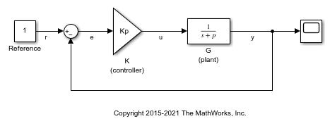
ex_scd_simple_fdbk モデルで基準信号 r からプラント出力 y への閉ループ伝達関数を取得します。

ex_scd_simple_fdbk モデルを開きます。

mdl = 'ex_scd_simple_fdbk';
open_system(mdl);

このモデルには次の項目が含まれています。

$\begin{array}{l}
K(s) = {K_p} = 3\\
G(s) = \frac{1}{{s + 5}}
\end{array}$

モデルの slLinearizer インターフェイスを作成します。

sllin = slLinearizer(mdl);

基準信号 r からプラント出力 y への閉ループ伝達関数を取得するには、両方の点を sllin に追加します。

addPoint(sllin,{'r','y'});

r から y への閉ループ伝達関数を取得します。

sys = getIOTransfer(sllin,'r','y');
tf(sys)

ans =
 
  From input "r" to output "y":
    3
  -----
  s + 8
 
Continuous-time transfer function.

ソフトウェアは、r で線形化入力 dr を追加し、y で線形化出力を追加します。

sys は dr から y への伝達関数であり、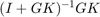 $(I+GK)^{-1}GK$ と等価です。

一時的ループ開始点の指定によるプラントモデルの取得

スクリプトを開く

ex_scd_simple_fdbk モデルで、プラントモデル伝達関数 G を取得します。

ex_scd_simple_fdbk モデルを開きます。

mdl = 'ex_scd_simple_fdbk';
open_system(mdl);

このモデルには次の項目が含まれています。

$\begin{array}{l}
K(s) = {K_p} = 3\\
G(s) = \frac{1}{{s + 5}}.
\end{array}$

モデルの slLinearizer インターフェイスを作成します。

sllin = slLinearizer(mdl);

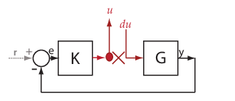
プラントモデルの伝達関数を取得するには、入力ポイントとして u、出力ポイントとして y を使用します。フィードバックの影響を取り除くには、ループを中断しなければなりません。ループは、u、e、または y で中断できます。この例では、u でループを中断します。これらの点を sllin に追加します。

addPoint(sllin,{'u','y'});

プラントモデル伝達関数を取得します。

sys = getIOTransfer(sllin,'u','y','u');
tf(sys)

ans =
 
  From input "u" to output "y":
    1
  -----
  s + 5
 
Continuous-time transfer function.

2 番目の入力引数で入力として u を指定し、4 番目の入力引数で一時的ループ開始点として u を指定します。

sys は du から y への伝達関数であり、と等価です。

特定のパラメーター組み合わせでの開ループ応答伝達関数の取得

スクリプトを開く

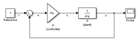
複数の伝達関数に対して scdcascade モデルをバッチ線形化するとします。ほとんどの線形化では、C2 コントローラーの比例ゲイン (Kp2) と積分ゲイン (Ki2) を 10% の範囲で変化させます。この例では、Kp2 および Ki2 の最大値について、e2 から y2 への内側のループの開ループ応答伝達関数を計算します。

scdcascade モデルを開きます。

mdl = 'scdcascade';
open_system(mdl)

モデルの slLinearizer インターフェイスを作成します。

sllin = slLinearizer(mdl);

C2 コントローラーの比例ゲイン (Kp2) および積分ゲイン (Ki2) を 10% の範囲で変化させます。

Kp2_range = linspace(0.9*Kp2,1.1*Kp2,3);
Ki2_range = linspace(0.9*Ki2,1.1*Ki2,5);

[Kp2_grid,Ki2_grid] = ndgrid(Kp2_range,Ki2_range);

params(1).Name = 'Kp2';
params(1).Value = Kp2_grid;

params(2).Name = 'Ki2';
params(2).Value = Ki2_grid;

sllin.Parameters = params;

内側のループの開ループ伝達関数を計算するには、e2 および y2 を解析ポイントとして使用します。外側のループの影響を取り除くには、e2 でループを中断します。解析ポイントとして e2 と y2 を sllin に追加します。

addPoint(sllin,{'e2','y2'})

Ki2 および Kp2 の最大値のインデックスを決定します。

mdl_index = params(1).Value == max(Kp2_range) & params(2).Value == max(Ki2_range);

e2 から y2 への開ループ伝達関数を取得します。

sys = getIOTransfer(sllin,'e2','y2','e2',mdl_index);

入力/出力伝達関数からのオフセットの取得

スクリプトを開く

Simulink® モデルを開きます。

mdl = 'scdcascade';
open_system(mdl)

線形化オプションセットを作成し、StoreOffsets オプションを設定します。

opt = linearizeOptions('StoreOffsets',true);

slLinearizer インターフェイスを作成します。

sllin = slLinearizer(mdl,opt);

解析ポイントを追加して閉ループ伝達関数を計算します。

addPoint(sllin,{'r','y1m'});

入力/出力伝達関数を計算し、対応する線形化オフセットを取得します。

[sys,info] = getIOTransfer(sllin,'r','y1m');

オフセットを表示します。

info.Offsets

ans = 

  struct with fields:

            dx: [6×1 double]
             x: [6×1 double]
             u: 1
             y: 0
    OutputName: {'y1m'}
     InputName: {'r'}
     StateName: {6×1 cell}
            Ts: 0

入力引数

すべて折りたたむ

`s` — Simulink^® モデルへのインターフェイス
`slLinearizer` インターフェイス | `slTuner` インターフェイス

Simulink モデルへのインターフェイス。slLinearizer インターフェイスまたは slTuner インターフェイスとして指定します。

`in` — 入力解析ポイント信号名
文字ベクトル | string | 文字ベクトルの cell 配列 | string 配列

入力解析ポイント信号名。以下で指定します。

文字ベクトルまたは string — 解析ポイント信号名。
解析ポイントに関連付けられた信号名を確認するには、s と入力します。MATLAB^® コマンドウィンドウに s の内容が表示されます。これには、解析ポイント信号名、ブロック名および端子番号が含まれます。解析ポイントに信号名がなく、ブロック名と端子番号のみがあるとします。ブロック名として in を指定できます。s の解析ポイントのリストにないポイントを使用するには、最初に addPoint を使用してポイントを追加します。
完全な信号名またはブロック名の一意的に一致する部分として in を指定できます。解析ポイントの完全な信号名が 'LoadTorque' であるとします。'Torque' が s の他の解析ポイントの信号名の一部でない限り、in を 'Torque' と指定できます。
たとえば、in = 'y1m' とします。
文字ベクトルの cell 配列または string 配列 — 複数の解析ポイント名を指定します。たとえば、in = {'y1m','y2m'} とします。

`out` — 出力解析ポイント信号名
文字ベクトル | string | 文字ベクトルの cell 配列 | string 配列

出力解析ポイント信号名。以下で指定します。

文字ベクトルまたは string — 解析ポイント信号名。
解析ポイントに関連付けられた信号名を確認するには、s と入力します。MATLAB コマンドウィンドウに s の内容が表示されます。これには、解析ポイント信号名、ブロック名および端子番号が含まれます。解析ポイントに信号名がなく、ブロック名と端子番号のみがあるとします。ブロック名として out を指定できます。s の解析ポイントのリストにないポイントを使用するには、最初に addPoint を使用してポイントを追加します。
完全な信号名またはブロック名の一意的に一致する部分として out を指定できます。解析ポイントの完全な信号名が 'LoadTorque' であるとします。'Torque' が s の他の解析ポイントの信号名の一部でない限り、out を 'Torque' と指定できます。
たとえば、out = 'y1m' とします。
文字ベクトルの cell 配列または string 配列 — 複数の解析ポイント名を指定します。たとえば、out = {'y1m','y2m'} とします。

`temp_opening` — 一時的開始点信号名
文字ベクトル | string | 文字ベクトルの cell 配列 | string 配列

一時的開始点信号名。以下で指定します。

文字ベクトルまたは string — 解析ポイント信号名。
temp_opening では、s の解析ポイントのリストに存在する解析ポイントを指定しなければなりません。解析ポイントに関連付けられた信号名を確認するには、s と入力します。MATLAB コマンドウィンドウに s の内容が表示されます。これには、解析ポイント信号名、ブロック名および端子番号が含まれます。解析ポイントに信号名がなく、ブロック名と端子番号のみがあるとします。ブロック名として temp_opening を指定できます。s の解析ポイントのリストにないポイントを使用するには、最初に addPoint を使用してポイントを追加します。
完全な信号名またはブロック名の一意的に一致する部分として temp_opening を指定できます。解析ポイントの完全な信号名が 'LoadTorque' であるとします。'Torque' が s の他の解析ポイントの信号名の一部でない限り、temp_opening を 'Torque' と指定できます。
たとえば、temp_opening = 'y1m' とします。
文字ベクトルの cell 配列または string 配列 — 複数の解析ポイント名を指定します。たとえば、temp_opening = {'y1m','y2m'} とします。

`ios` — 線形化 I/O
線形化 I/O オブジェクト

linio を使用して作成された線形化 I/O。線形化 I/O オブジェクトとして指定します。

ios は、s の解析ポイントのリストにある信号を指定しなければなりません。解析ポイントのリストを表示するには、s と入力します。s の解析ポイントのリストにないポイントを使用するには、最初に addPoint を使用してポイントをリストに追加しなければなりません。

以下に例を示します。

ios(1) = linio('scdcascade/setpoint',1,'input');
ios(2) = linio('scdcascade/Sum',1,'output');

ここでは、ios(1) で入力を指定し、ios(2) で出力を指定します。

`mdl_index` — 対象の線形化のインデックス
論理値の配列 | 正の整数のベクトル

対象の線形化のインデックス。以下で指定します。

論理値の配列 — 対象の線形化の論理配列のインデックス。2 つのパラメーター par1 と par2 を変化させ、par1 > 0.5 と par2 <= 5 の組み合わせで線形化を抽出するとします。使用:
```
params = s.Parameters;
mdl_index = params(1).Value>0.5 & params(2).Value <= 5;
```
式 params(1).Value>0.5 & params(2).Value<5 は論理インデックス付けを使用して、logical 配列を返します。この logical 配列は、params(1).Value および params(2).Value と同じサイズです。各エントリには、params(1).Value および params(2).Value 内の対応するエントリの式の論理評価が含まれます。
正の整数のベクトル — 対象の線形化の線形インデックス。2 つのパラメーター par1 と par2 を変化させ、par1 > 0.5 と par2 <= 5 の組み合わせで線形化を抽出するとします。使用:
```
params = s.Parameters;
mdl_index = find(params(1).Value>0.5 & params(2).Value <= 5);
```
式 params(1).Value>0.5 & params(2).Value<5 は logical 配列を返します。find はその logical 配列の true の各エントリの線形インデックスを返します。

出力引数

すべて折りたたむ

`linsys` — 指定された I/O の伝達関数
状態空間モデル

指定された I/O の伝達関数。以下の説明のように返されます。

s.Parameters および s.OperatingPoints を設定していない場合、ソフトウェアは既定のモデルパラメーター値を使用して linsys を計算します。ソフトウェアはモデルの初期条件を線形化の操作点として使用します。linsys は状態空間モデルとして返されます。
s.Parameters のみを設定している場合、ソフトウェアはそれぞれのパラメーターグリッド点の線形化を計算します。linsys は、パラメーターグリッドと同じサイズの状態空間モデル配列として返されます。
s.OperatingPoints のみを設定している場合、ソフトウェアは指定されたそれぞれの操作点の線形化を計算します。linsys は、s.OperatingPoints と同じサイズの状態空間モデル配列として返されます。
s.Parameters を設定しており、s.OperatingPoints を単一の操作点として指定している場合、ソフトウェアはそれぞれのパラメーターグリッド点の線形化を計算します。ソフトウェアは、指定された操作点を線形化の操作点として使用します。linsys は、パラメーターグリッドと同じサイズの状態空間モデル配列として返されます。
s.Parameters を設定しており、s.OperatingPoints を複数の操作点オブジェクトとして指定している場合、ソフトウェアはそれぞれのパラメーターグリッド点の線形化を計算します。s.OperatingPoints は s.Parameters で指定されたパラメーターグリッドと同じサイズでなければなりません。ソフトウェアは、対応する操作点およびパラメーターグリッド点を使用してそれぞれの線形化を計算します。linsys はパラメーターグリッドと同じサイズの状態空間モデル配列として返されます。
s.Parameters を設定しており、s.OperatingPoints を複数のシミュレーションスナップショット時間として指定している場合、ソフトウェアはスナップショット時間とパラメーターグリッド点のそれぞれの組み合わせに対してモデルをシミュレートして線形化します。サイズ p のパラメーターグリッドと N 個のスナップショット時間を指定するとします。linsys は、サイズが N 行 p 列の状態空間モデル配列として返されます。

ほとんどのモデルでは、linsys は ss オブジェクトまたは ss オブジェクトの配列として返されます。ただし、モデルの in と out で定義された線形化パスに次のいずれかのブロックが含まれている場合、linsys は指定されたタイプの状態空間モデルを返します。

ブロック	`linsys` のタイプ
`genss` オブジェクトまたは調整可能なモデルオブジェクトとして指定された置換をもつブロック	`genss`
`uss` などの不確かさをもつモデルとして指定された置換をもつブロック	`uss` (Robust Control Toolbox)
Sparse Second Order ブロック	`mechss`
スパースモデルに線形化するように構成された Descriptor State-Space ブロック	`sparss`

`info` — 線形化の情報
構造体

線形化の情報。次のフィールドを含む構造体として返されます。

`Offsets` — 線形化のオフセット
`[]` (既定値) | 構造体 | 構造体配列

線形化のオフセット。s.Options.StoreOffsets が false の場合は [] として返されます。それ以外の場合、Offsets は次のいずれかとして返されます。

linsys が単一の状態空間モデルの場合、Offsets は構造体になります。
linsys が状態空間モデルの配列の場合、Offsets は linsys と同じ次元をもつ構造体配列になります。

オフセットの各構造体には次のフィールドがあります。

フィールド	説明
`x`	線形化に使用された状態のオフセット。長さ n_x の列ベクトルとして返されます。n_x は `linsys` にある状態の数です。
`y`	線形化に使用された出力のオフセット。長さ n_y の列ベクトルとして返されます。n_y は `linsys` にある出力の数です。
`u`	線形化に使用された入力のオフセット。長さ n_u の列ベクトルとして返されます。n_u は `linsys` にある入力の数です。
`dx`	連続時間システムの微分オフセット、または離散時間システムの更新された状態値。長さ n_x の列ベクトルとして返されます。
`StateName`	状態名。`linsys.StateName` の名前に一致する n_x 個の要素をもつ cell 配列として返されます。
`InputName`	入力名。`linsys.InputName` の名前に一致する n_u 個の要素をもつ cell 配列として返されます。
`OutputName`	出力名。`linsys.OutputName` の名前に一致する n_y 個の要素をもつ cell 配列として返されます。
`Ts`	線形化されたシステムのサンプル時間。`linsys.Ts` のサンプル時間に一致するスカラーとして返されます。連続時間システムの場合、`Ts` は `0` です。

Offsets が構造体配列の場合、オフセットを使用して LPV System ブロックを構成できます。これを行うには、まず getOffsetsForLPV を使用してオフセットを必要な形式に変換します。例については、LTI システムの配列を使用した非線形動作の近似を参照してください。

`Advisor` — 線形化の診断情報
`[]` (既定値) | `LinearizationAdvisor` オブジェクト | `LinearizationAdvisor` オブジェクトの配列

線形化の診断情報。s.Options.StoreAdvisor が false の場合は [] として返されます。それ以外の場合、Advisor は次のいずれかとして返されます。

linsys が単一の状態空間モデルの場合、Advisor は LinearizationAdvisor オブジェクトになります。
linsys が状態空間モデルの配列の場合、Advisor は linsys と同じ次元をもつ LinearizationAdvisor オブジェクトの配列になります。

LinearizationAdvisor オブジェクトは個々の線形化ブロックについての線形化の診断情報を格納します。LinearizationAdvisor オブジェクトを使用して線形化の結果をトラブルシューティングする例は、コマンドラインを使用した線形化の結果のトラブルシューティングを参照してください。

詳細

すべて折りたたむ

伝達関数

"伝達関数" とは、線形化出力ポイントにおける線形化入力に対する LTI システムの応答です。伝達関数で線形解析を実行し、システムの安定性、時間領域の特性または周波数領域の特性を理解します。

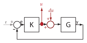
与えられたブロック線図で複数の伝達関数を計算できます。ex_scd_simple_fdbk モデルを考えます。

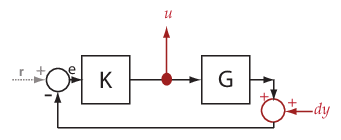
基準入力信号からプラント出力信号への伝達関数を計算できます。"基準入力" ("設定点" とも呼ばれる) r は Reference ブロックで発生し、"プラント出力" y は G ブロックで発生します。この伝達関数は、"閉ループ全体の" 伝達関数とも呼ばれます。この伝達関数を計算するために、ソフトウェアは、r で線形化入力 dr を追加し、y で線形化出力を追加します。

ソフトウェアは、dr から y への伝達関数として閉ループ全体の伝達関数を計算します。これは、(I+GK)^-1GK と同じです。

r から y への伝達関数が dr から y への伝達関数と同じになることを確認します。

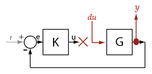
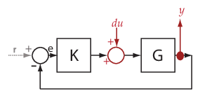
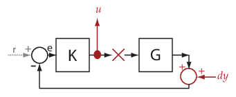
プラント入力 u からプラント出力 y への "プラント伝達関数" を計算できます。プラントのダイナミクスをフィードバックループの影響から切り離すには、y、e、または図のように u にループの中断 (つまり "開始点") を導入します。

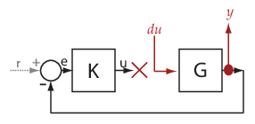
ソフトウェアはループを中断し、u で線形化入力 du を追加し、y で線形化出力を追加します。このプラント伝達関数は、du から y への伝達関数 (G) と同じです。

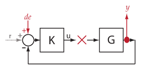
同様に、"コントローラー伝達関数" を取得するには、コントローラー入力 e からコントローラー出力 u への伝達関数を計算します。y、e または u でフィードバックループを中断します。

getIOTransfer を使用して、さまざまな開ループまたは閉ループの伝達関数を取得できます。伝達関数を設定するには、任意の組み合わせで入力、出力および開始点 (一時的または永続的) として解析ポイントを指定します。ソフトウェアはそれぞれの組み合わせを一意的に処理します。次のコードについて考えます。これは、解析ポイント u を使用して伝達関数を取得するいくつかの方法を示します。

sllin = slLinearizer('ex_scd_simple_fdbk')

addPoint(sllin,{'u','e','y'})

T0 = getIOTransfer(sllin,'e','y','u');
T1 = getIOTransfer(sllin,'u','y');
T2 = getIOTransfer(sllin,'u','y','u');
T3 = getIOTransfer(sllin,'y','u');
T4 = getIOTransfer(sllin,'y','u','u');
T5 = getIOTransfer(sllin,'u','u'); 
T6 = getIOTransfer(sllin,'u','u','u');

T0 では、u でループの中断を指定します。T1 では、u で入力のみを指定します。T2 では、u で入力および開始点 ("開ループの入力" とも呼ばれる) を指定します。T3 では、u で出力のみを指定します。T4 では、u で出力および開始点 ("開ループの出力" とも呼ばれる) を指定します。T5 では、u で入力および出力 ("相補感度ポイント" とも呼ばれる) を指定します。T6 では、u で入力、出力および開始点 ("ループ伝達ポイント" とも呼ばれる) を指定します。次の表は、getIOTransfer が解析ポイントを処理する方法を示します。ここでは、u のさまざまな使用方法に注目します。

`u` の指定内容	`getIOTransfer` による解析ポイントの処理	伝達関数
ループの中断コード例: T0 = getIOTransfer(... sllin,'e','y','u')	ソフトウェアは `u` で信号の流れを切断し、線形化入力 `de` を `e` に、線形化出力を `y` に追加します。`de` から `e` へのパスがないため、伝達関数はゼロになります。	$\begin{array}{l} \begin{array}{l} y = G 0 \\ \to y = 0 \end{array} \\ ∴ T_{0} = 0 \end{array}$
入力コード例: T1 = getIOTransfer(... sllin,'u','y')	ソフトウェアは、`u` に線形化入力 `du` を、`y` に線形化出力を追加します。	$\begin{array}{l} y = G (d u - K y) \\ \to y = G d u - G K y \\ \to (I + G K) y = G d u \\ \to y = {(I + G K)}^{- 1} G d u \\ ∴ T_{1} = {(I + G K)}^{- 1} G \end{array}$
開ループの入力コード例: T2 = getIOTransfer(... sllin,'u','y','u')	ソフトウェアは `u` で信号の流れを切断して線形化入力 `du` を追加し、`y` に線形化出力を追加します。	$\begin{array}{l} y = G (d u + 0) \\ \begin{array}{l} \to y = G d u \\ ∴ T_{2} = G \end{array} \end{array}$
出力コード例: T3 = getIOTransfer(... sllin,'y','u')	ソフトウェアは、`y` で線形化入力 `dy` を、`u` で線形化出力を追加します。	$\begin{array}{l} u = - K (d y + G u) \\ \to u = - K d y - K G u \\ \to (I + K G) u = - K d y \\ \to u = - {(I + K G)}^{- 1} K d y \\ ∴ T_{3} = - {(I + K G)}^{- 1} K \end{array}$
開ループの出力コード例: T4 = getIOTransfer(... sllin,'y','u','u')	ソフトウェアは `y` で線形化入力 `dy` を追加し、`u` で線形化出力を追加して信号の流れを切断します。	$\begin{array}{l} u = - K (d y + G 0) \\ \begin{array}{l} \to u = - K d y \\ ∴ T_{4} = - K \end{array} \end{array}$
相補感度ポイントコード例: T5 = getIOTransfer(... sllin,'u','u') ヒント `getCompSensitivity` を使用して相補感度関数を取得することもできます。	ソフトウェアは、`u` で線形化出力および線形化入力 `du` を追加します。	$\begin{array}{l} u = - K G (d u + u) \\ \to u = - K G d u - K G u \\ \to (I + K G) u = - K G d u \\ \begin{array}{l} \to u = - {(I + K G)}^{- 1} K G d u \\ ∴ T_{5} = - {(I + K G)}^{- 1} K G \end{array} \end{array}$
ループ伝達関数の点コード例: T6 = getIOTransfer(... sllin,'u','u','u') ヒント `getLoopTransfer` を使用してループ伝達関数を取得することもできます。	ソフトウェアは `u` で線形化出力を追加して、ループを中断し、線形化入力 `du` を追加します。	$\begin{array}{l} u = - K G (d u + 0) \\ \to u = - K G d u \\ ∴ T_{6} = - K G \end{array}$

ソフトウェアは、伝達関数を計算する際に Simulink モデルを変更しません。

解析ポイント

"解析ポイント" は、slLinearizer と slTuner インターフェイスで使用され、モデル内で線形解析と制御システムの調整に関連する箇所を示します。解析ポイントは、getIOTransfer、getLoopTransfer、getSensitivity、getCompSensitivity などの線形化コマンドの入力として使用します。線形化コマンドの入力として、解析ポイントによりモデル内の開ループまたは閉ループの伝達関数を指定できます。また、systune などのコマンドを使って制御システムを調整する際に、解析ポイントを使用して設計要件を指定することもできます。

"場所" とは、モデル内の特定のブロック出力端子か、そのような出力端子にあるバス要素を指します。便宜上、この端子から発信する信号の名前を使って解析ポイントを示すことができます。

解析ポイントは、slLinearizer または slTuner インターフェイス s に対して、インターフェイスの作成時に追加できます。以下に例を示します。

s = slLinearizer('scdcascade',{'u1','y1'});

また、addPoint コマンドを使用することもできます。

s のすべての解析ポイントを表示するには、コマンドプロンプトで s と入力してインターフェイスの内容を表示します。s の各解析ポイントの表示には、ブロック名、端子番号、およびこの解析ポイントから発信される信号の名前が含まれます。getPoints を使用して、すべての解析ポイントのリストをプログラムで取得することもできます。

解析ポイントの使用方法の詳細については、制御システムの解析と設計における対象信号のマークおよびバッチ線形化用に対象の信号をマークするを参照してください。

永続的な開始点

"永続的な開始点" とは、slLinearizer および slTuner インターフェイスで使用され、ソフトウェアがモデル内で信号の流れを中断する箇所を示します。線形化および調整時に、これらの開始点が強制的に適用されます。永続的な開始点は、ある特定のモデルコンポーネントを分離するために使用します。航空機のダイナミクスを取得する大規模なモデルがあり、機体にのみ線形解析を実行するとします。永続的な開始点を使用すれば、このモデルの他のコンポーネントをすべて除外できます。モデル内にカスケード式ループがあり、特定のループを解析する場合などにも使用できます。

"場所" とは、モデル内の特定のブロック出力端子を指します。便宜上、この端子から発信する信号の名前を使って開始点を示すことができます。

永続的な開始点は、slLinearizer または slTuner インターフェイス s に対して、インターフェイスの作成時に追加するか、addOpening コマンドを使用して追加できます。永続的な開始点のリストから場所を削除するには、removeOpening コマンドを使用します。

s のすべての開始点を表示するには、コマンドプロンプトで s と入力してインターフェイスの内容を表示します。s のそれぞれの永続的な開始点の表示には、ブロック名、端子番号、およびこの場所から発信される信号の名前が含まれます。getOpenings を使用して、すべての永続的なループ開始点のリストをプログラムで取得することもできます。

バージョン履歴

R2013b で導入

すべて展開する

R2020b: Simulink モデルをスパース状態空間モデルに線形化

Sparse Second Order ブロックまたは Descriptor State-Space ブロックを含む Simulink モデルからスパースモデルを線形化および取得できます。

Simulink モデルで Sparse Second Order を使用する場合の mechss モデル。
Descriptor State-Space ブロックを使用し、[スパースモデルに線形化する] ブロックパラメーターを選択する場合の sparss モデル。

詳細については、スパースモデルの基礎を参照してください。例については、スパース 2 次モデルオブジェクトへの Simulink モデルの線形化を参照してください。

R2016b: 線形化時にモデルの入力、出力、状態、および状態微分の操作点のオフセットを計算

Simulink モデルを線形化する際にモデルの入力、出力、状態、および状態微分の操作点のオフセットを計算できます。3 つのオフセットにより、線形パラメーター変動 (LPV) システムの作成が合理化します。

操作点のオフセットを取得するには、まず linearizeOptions または slTunerOptions オブジェクトを作成して、StoreOffsets オプションを true に設定します。次に、モデルの slLinearizer または slTuner インターフェイスを作成します。

getIOTransfer の info 出力引数からオフセットを抽出し、関数 getOffsetsForLPV を使用して LPV System ブロックの必要な形式に変換できます。

参考

getIOTransfer

構文

説明

例

基準からプラント出力への閉ループ伝達関数の取得

一時的ループ開始点の指定によるプラント モデルの取得

特定のパラメーター組み合わせでの開ループ応答伝達関数の取得

入力/出力伝達関数からのオフセットの取得

入力引数

s — Simulink® モデルへのインターフェイス slLinearizer インターフェイス | slTuner インターフェイス

in — 入力解析ポイント信号名 文字ベクトル | string | 文字ベクトルの cell 配列 | string 配列

out — 出力解析ポイント信号名 文字ベクトル | string | 文字ベクトルの cell 配列 | string 配列

temp_opening — 一時的開始点信号名 文字ベクトル | string | 文字ベクトルの cell 配列 | string 配列

ios — 線形化 I/O 線形化 I/O オブジェクト

mdl_index — 対象の線形化のインデックス 論理値の配列 | 正の整数のベクトル

出力引数

linsys — 指定された I/O の伝達関数 状態空間モデル

info — 線形化の情報 構造体

Offsets — 線形化のオフセット [] (既定値) | 構造体 | 構造体配列

Advisor — 線形化の診断情報 [] (既定値) | LinearizationAdvisor オブジェクト | LinearizationAdvisor オブジェクトの配列

詳細

伝達関数

解析ポイント

永続的な開始点

バージョン履歴

R2020b: Simulink モデルをスパース状態空間モデルに線形化

R2016b: 線形化時にモデルの入力、出力、状態、および状態微分の操作点のオフセットを計算

参考

トピック

一時的ループ開始点の指定によるプラントモデルの取得

`s` — Simulink^® モデルへのインターフェイス
`slLinearizer` インターフェイス | `slTuner` インターフェイス

`in` — 入力解析ポイント信号名
文字ベクトル | string | 文字ベクトルの cell 配列 | string 配列

`out` — 出力解析ポイント信号名
文字ベクトル | string | 文字ベクトルの cell 配列 | string 配列

`temp_opening` — 一時的開始点信号名
文字ベクトル | string | 文字ベクトルの cell 配列 | string 配列

`ios` — 線形化 I/O
線形化 I/O オブジェクト

`mdl_index` — 対象の線形化のインデックス
論理値の配列 | 正の整数のベクトル

`linsys` — 指定された I/O の伝達関数
状態空間モデル

`info` — 線形化の情報
構造体

`Offsets` — 線形化のオフセット
`[]` (既定値) | 構造体 | 構造体配列

`Advisor` — 線形化の診断情報
`[]` (既定値) | `LinearizationAdvisor` オブジェクト | `LinearizationAdvisor` オブジェクトの配列