このページの内容は最新ではありません。最新版の英語を参照するには、ここをクリックします。

ゼロクロッシング検出

可変ステップ ソルバーは、変数がゆっくり変化するときにはタイム ステップ サイズを増加させ、急速に変化するときには減少させて、タイム ステップ サイズを動的に調整します。この動作によってソルバーが不連続点付近で小さいステップを取りますが、これは変数の変化が急であるためです。このため精度は向上しますが、シミュレーション時間が余分にかかることがあります。

Simulink^® はゼロクロッシング検出という手法を使用して、過度に小さいタイム ステップを取ることなく正確に不連続点を特定します。この技法を使うとシミュレーション実行時間は短縮されますが、意図した完了時間前に一部のシミュレーションが停止することがあります。

この目的のため、Simulink は、非適応アルゴリズムと適応アルゴリズムという 2 つのアルゴリズムを使用します。これらの技法の詳細については、ゼロクロッシング アルゴリズムを参照してください。

シミュレーションにおける過度のゼロクロッシング検出の影響

この例では、2 つの Integrator ブロックを使用して跳ねるボールのダイナミクスをモデル化するモデル example_bounce_two_integrators を使用して、シミュレーションにおける過度のゼロクロッシングの影響を示します。パフォーマンス上の理由から、可能であれば、2 つの異なる Integrator ブロックよりも Second-Order Integrator ブロックを使用する方が推奨されます。Second-Order Integrator ブロックを使用して跳ねるボールのダイナミクスをモデル化する方法を示す例については、跳ねるボールのシミュレーションを参照してください。

モデル example_bounce_two_integrators を開きます。

mdl = "example_bounce_two_integrators";
open_system(mdl)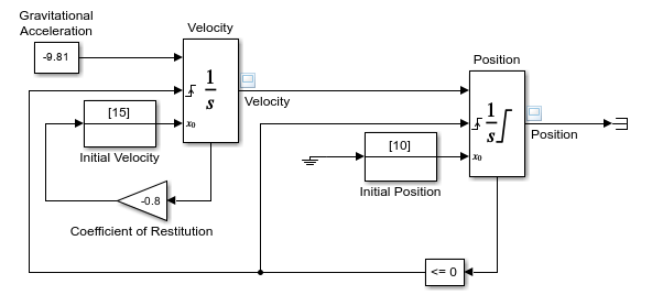

過度のゼロクロッシング検出の影響を確認するには、非適応ゼロクロッシング検出アルゴリズムを使用するようにモデルを構成します。

1. [コンフィギュレーション パラメーター] ダイアログ ボックスを開くには、Simulink® ツールストリップの [モデル化] タブの [設定] で [モデル設定] をクリックします。

2. [コンフィギュレーション パラメーター] ダイアログ ボックスの [ソルバー] ペインで、[ソルバーの詳細] を展開します。

3. [ソルバーの詳細] の [ゼロクロッシング オプション] で、[アルゴリズム] パラメーターを [Nonadaptive] に設定します。

4. [OK] をクリックします。

あるいは、set_param 関数を使用して ZeroCrossAlgorithm パラメーターを Nonadaptive に設定します。

set_param(mdl,ZeroCrossAlgorithm="Nonadaptive")

終了時間を 20 秒にしてモデルのシミュレーションを実行します。

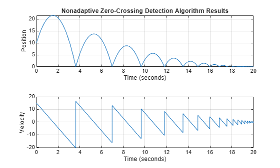
nonadaptive = sim(mdl,StopTime="20");

跳ねるボールの位置と速度をプロットします。跳ね返るたびに最大高さと最大速度が減少します。

nonadaptivePosition = getElement(nonadaptive.yout,"Position").Values;
nonadaptiveVelocity = getElement(nonadaptive.yout,"Velocity").Values;

tiledlayout(2,1)
ax1 = nexttile;
plot(nonadaptivePosition)
grid(ax1,"on")
title("Nonadaptive Zero-Crossing Detection Algorithm Results")
ax2 = nexttile;
plot(nonadaptiveVelocity)
grid(ax2,"on")
title("")

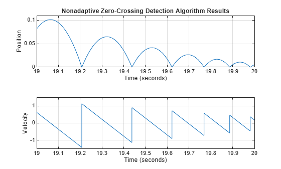
シミュレーション結果の最後の 1 秒のみをプロットします。シミュレーションの最後の 1 秒で、速度の値はゼロに近くなります。

tiledlayout(2,1)
ax1 = nexttile;
plot(nonadaptivePosition)
grid(ax1,"on")
title("Nonadaptive Zero-Crossing Detection Algorithm Results")
axis([19 20 0 0.11])
ax2 = nexttile;
plot(nonadaptiveVelocity)
grid(ax2,"on")
title("")
axis([19 20 -1.5 1.5])

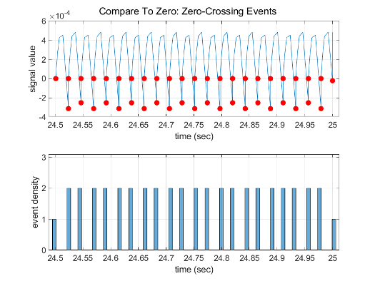
位置と速度の値がゼロに近づくにつれて、跳ね返りの時間は短くなります。ボールが跳ねるたびに、位置と速度の両方の信号がゼロクロッシングをもちます。跳ね返りの時間が短くなるにつれて、ゼロクロッシングの頻度は高くなります。

モデルを再度シミュレートします。今回は終了時間を 25 秒にしてシミュレーションを実行し、シミュレーションでゼロクロッシングの頻度の増加が非適応ゼロクロッシング アルゴリズムによってどのように処理されるかを確認します。CaptureErrors パラメーターを有効にして、頻繁にゼロクロッシングが検出されることでシミュレーション時に実行時エラーが発生しても sim 関数が確実に結果を返すようにします。

nonadaptive25 = sim(mdl,StopTime="25",CaptureErrors="on");

シミュレーションが停止した理由を確認するには、シミュレーション メタデータ内の実行情報を調べます。

st = nonadaptive25.SimulationMetadata.ExecutionInfo.StopEventDescription

st = 
    'Simulink will stop the simulation of model 'example_bounce_two_integrators' because the 2 zero crossing signal(s) identified below caused 1000 consecutive zero crossing events in time interval between 20.357636989536076 and 20.357636990631594.
      --------------------------------------------------------------------------------
     Number of consecutive zero-crossings : 1000
                Zero-crossing signal name : RelopInput
                               Block type : RelationalOperator
                               Block path : 'example_bounce_two_integrators/Compare To Zero/Compare'
     --------------------------------------------------------------------------------
     --------------------------------------------------------------------------------
     Number of consecutive zero-crossings : 500
                Zero-crossing signal name : x Lower Saturation
                               Block type : Integrator
                               Block path : 'example_bounce_two_integrators/Position'
     --------------------------------------------------------------------------------
      '

シミュレーションが停止したのは、モデル内の Compare To Zero および Position という名前のブロックであまりにも多くの連続ゼロクロッシング イベントが検出されたことで実行時エラーが発生したためです。

非適応ゼロクロッシング検出アルゴリズムは、検出されたすべてのゼロクロッシング イベントを囲い込んで、シミュレーション中に発生したすべてのゼロクロッシングの位置を特定します。非適応アルゴリズムは多くのモデルやシミュレーションに適しますが、高度なチャタリングや Zeno 動作があるシステムで非適応アルゴリズムを使用すると、タイム ステップの間隔が非常に短くなり、シミュレーションが非常に遅くなることがあります。

適応ゼロクロッシング検出アルゴリズムは、ゼロクロッシング信号値が十分にゼロに近い場合、および連続ゼロクロッシングの数が上限に達した場合に、囲い込みを中止します。過度の連続ゼロクロッシングが原因で適応アルゴリズムが囲い込みを無効にした場合、既定では、シミュレーションはゼロクロッシング イベントの無視に関する警告を発行します。

適応ゼロクロッシング検出アルゴリズムを使用して、終了時間を 25 秒にしてモデルのシミュレーションを試します。ゼロクロッシングの無視に関する警告を非表示にするには、[無視されたゼロクロッシング] パラメーターを [none] に設定します。

1. [コンフィギュレーション パラメーター] ダイアログ ボックスの [ソルバー] ペインの [ゼロクロッシング オプション] で、[アルゴリズム] パラメーターを [Adaptive] に設定します。

2. [コンフィギュレーション パラメーター] ダイアログ ボックスの [診断] ペインで、省略記号をクリックして [詳細設定パラメーター] を展開します。次に、[無視されたゼロクロッシング] パラメーターを [none] に設定します。

あるいは、set_param 関数を使用して ZeroCrossAlgorithm パラメーターを Adaptive に、IgnoredZcDiagnostic パラメーターを none に設定します。

set_param(mdl,ZeroCrossAlgorithm="Adaptive",IgnoredZcDiagnostic="none")

終了時間を 25 秒にしてモデルのシミュレーションを再度実行します。CaptureErrors パラメーターを有効にして、頻繁にゼロクロッシングが検出されることでシミュレーション時に実行時エラーが発生しても sim 関数が確実に結果を返すようにします。

adaptive = sim(mdl,StopTime="25",CaptureErrors="on");

シミュレーションが停止した理由を確認するには、シミュレーション メタデータ内の実行情報を調べます。

st = adaptive.SimulationMetadata.ExecutionInfo.StopEventDescription

st = 
'Reached stop time of 25'

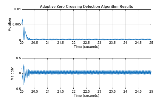
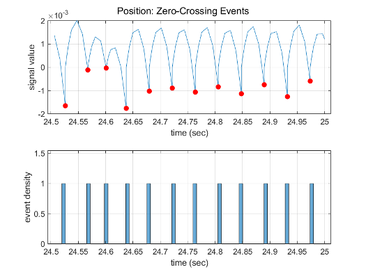
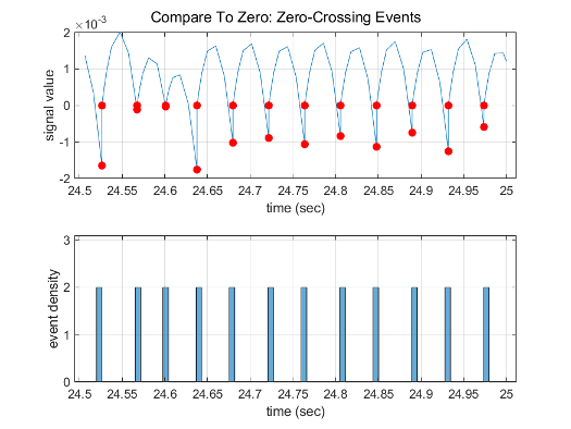
シミュレーションは、終了時間の 25 秒に達した後停止しました。跳ねるボールの位置と速度をプロットします。20 秒のシミュレーション時間中の結果は、非適応ゼロクロッシング検出アルゴリズムを使用した 20 秒のシミュレーションの結果と一致します。20 秒経過した後は、位置と速度の両方がゼロになるようです。

adaptivePosition = getElement(adaptive.yout,"Position").Values;
adaptiveVelocity = getElement(adaptive.yout,"Velocity").Values;

tiledlayout(2,1)
ax1 = nexttile;
plot(adaptivePosition)
grid(ax1,"on")
title("Adaptive Zero-Crossing Detection Algorithm Results")
ax2 = nexttile;
plot(adaptiveVelocity)
grid(ax2,"on")
title("")

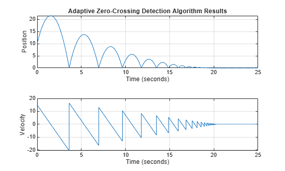
シミュレーション結果の最後の 5 秒のみをプロットします。結果はより完全であり、跳ねるボールのダイナミクスを制御する方程式の想定される解析解により近くなります。結果におけるチャタリングは、システムの状態の値がゼロに近づく際に数値シミュレーションで想定されるものです。

tiledlayout(2,1)
ax1 = nexttile;
plot(adaptivePosition)
grid(ax1,"on")
title("Adaptive Zero-Crossing Detection Algorithm Results")
axis([20 25 0 0.01])
ax2 = nexttile;
plot(adaptiveVelocity)
grid(ax2,"on")
title("")
axis([20 25 -0.5 0.5])

過度のゼロクロッシングの回避

次の表を使用して、モデルで過度のゼロクロッシング エラーを防ぎます。

変更のタイプ	変更の手順	利点
ゼロクロッシングの許可数を増やす	[コンフィギュレーション パラメーター] ダイアログ ボックスの [ソルバー] ペインの [連続的なゼロクロッシングの数] の値を増やします。	ゼロクロッシングを解決する時間が十分与えられます。
[信号のしきい値] を緩める	[コンフィギュレーション パラメーター] ダイアログ ボックスの [ソルバー] ペインで [アルゴリズム] プルダウンを [適応] を選択し、 [信号のしきい値] オプションの値を増やします。	ソルバーがゼロクロッシングを正確に検出するための必要時間を短くします。こうすることでシミュレーション時間を短縮し、過度の連続ゼロクロッシング エラー数を減らします。ただし、[信号のしきい値] を緩めると精度が低下する可能性があります。
[適応] アルゴリズムを使用する	[コンフィギュレーション パラメーター] ダイアログ ボックスの [ソルバー] ペインで [アルゴリズム] ドロップダウンから [適応] を選択します。	このアルゴリズムは、ゼロクロッシングのしきい値を動的に調整します。これにより、精度が向上し、検出される連続ゼロクロッシングの数が減ります。このアルゴリズムには、[時間の許容誤差] と [信号のしきい値] の両方を指定するオプションがあります。
特定のブロックでゼロクロッシング検出を無効にする	ブロックのパラメーター ダイアログ ボックスの [ゼロクロッシング検出を有効にする] チェック ボックスをオフにします。 [コンフィギュレーション パラメーター] ダイアログ ボックスの [ソルバー] ペインで [ゼロクロッシング コントロール] プルダウンから [ローカル設定を使用] を選択します。	ゼロクロッシング検出をローカルで無効にすると、特定のブロックでの過度の連続ゼロクロッシングによるシミュレーション停止を回避することができます。他のすべてのブロックには引き続きゼロクロッシング検出が有効で精度が向上します。
モデル全体でゼロクロッシング検出を無効にする	[コンフィギュレーション パラメーター] ダイアログ ボックスの [ソルバー] ペインで [ゼロクロッシング コントロール] プルダウンから [すべて無効] を選択します。	こうすると、モデルのあらゆる場所でゼロクロッシングが検出されなくなります。この結果、ゼロクロッシング検出が無効でモデルの精度は向上しません。
ode15s ソルバーを使用している場合は、数値微分式の順序を調整する	[コンフィギュレーション パラメーター] ダイアログ ボックスの [ソルバー] ペインで [Maximum order] プルダウンから値を選択します。	詳細については、Maximum orderを参照してください。
最大ステップ サイズを減らす	[コンフィギュレーション パラメーター] ダイアログ ボックスの [ソルバー] ペインの [最大ステップ サイズ] オプションに値を入力します。	ソルバーがゼロクロッシングの解決に必要とするステップ数が抑えられます。ただし、ステップ サイズを減らすとシミュレーション時間が増えます。適応アルゴリズムを使用している場合はほとんど必要ありません。

シミュレーターがゼロクロッシング イベントを見落とす場合

跳ねるボールのシミュレーションおよび2 個の跳ねるボール: 適応ゼロクロッシング位置の使用の bounce モデルと double-bounce モデルから、不連続点周辺の高周波変動 (「チャタリング」) が、シミュレーションの早期停止を引き起こす可能性があることがわかります。

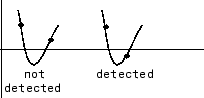
また、ソルバーの許容誤差が大きすぎる場合もソルバーがゼロクロッシングを完全に見落とすことがあります。これは、ゼロクロッシング検出技法では、信号の値によって符号が変更されたかどうかがメジャー タイム ステップの後にチェックされることが原因です。符号変更はゼロクロッシングが発生したことを示し、ゼロクロッシング アルゴリズムは正確なクロッシングの時間を探します。しかし、ゼロクロッシングがある 1 つのタイム ステップの開始時と終了時で値の符号変化がない場合を想定してみましょう。このような場合、ソルバーがゼロクロッシング部を検出できずに、その位置を横切ってしまいます。

次の図は、ゼロを横切る信号を示しています。最初の例では、タイム ステップ間で符号が変わっていないため、積分はこのイベントを飛び越えてしまいます。2 番目の例では、ソルバーが符号の変化を検出し、したがってゼロクロッシング イベントを検出します。

bounce モデルの 2 つの積分器実装について考えてみます。

[ソルバー プロファイラー] を使用してシミュレーションの最後の 0.5 秒をプロファイリングすると、シミュレーションでは Compare To Zero ブロックで 44 のゼロクロッシングを検出し、Position ブロックの出力で 22 のイベントを検出することがわかります。

[相対許容誤差] パラメーターの値を、既定の 1e-3 ではなく 1e-2 に増やします。このパラメーターは [コンフィギュレーション パラメーター] ダイアログ ボックスの [ソルバー] ペインの [ソルバーの詳細] セクション、または set_param を使用して RelTol を '1e-2' として指定することで変更できます。

新しいソルバーの相対許容誤差を使用してシミュレーションの最後の 0.5 秒をプロファイリングすると、Compare To Zero ブロックでは 24 のゼロクロッシング イベント、Position ブロックの出力では 12 イベントのみが検出されることがわかります。

ブロックでのゼロクロッシング検出

ブロックはゼロクロッシング変数のセットを登録できます。それらは、不連続点をもつ状態変数の関数です。ゼロクロッシング関数は、対応する不連続が生じるとき正または負の値からゼロを渡します。登録されたゼロクロッシング変数は各シミュレーション ステップの最後に更新され、符号が変わった変数はゼロクロッシング イベントとして特定されます。

ゼロクロッシングが検出された場合、Simulink ソフトウェアは符号が変化した変数の前の値と現在の値の間で内挿を行い、ゼロクロッシングの時間 (不連続点) を推定します。

メモ

ゼロクロッシング検出アルゴリズムは、データ型が double の信号に対してのみ、ゼロクロッシング イベントをまとめることができます。

ゼロクロッシングを登録するブロック

次の表で、ゼロクロッシングを登録するブロックのリストとブロックがどのようにしてゼロクロッシングを使用するかについて説明します。

ブロック	ゼロクロッシングの検出の数
Abs	1: 正方向または負方向に向かう入力信号がゼロと交わる瞬間を検出。
Backlash	2: 1 つは上限しきい値に到達する瞬間を検出し、もう 1 つは下限しきい値に到達する瞬間を検出。
Compare To Constant	1: 信号が定数と等しくなる瞬間を検出。
Compare To Zero	1: 信号がゼロと等しくなる瞬間を検出。
Dead Zone	2: 1 つは不感帯に入る瞬間 (入力信号から下限値を差し引いたもの) を検出し、もう 1 つは不感帯から出る瞬間 (入力信号から上限値を差し引いたもの) を検出。
Enable	1: イネーブル端子が Subsystem ブロックの中にあるときに、ゼロクロッシング検出機能を提供。詳細については、Enabled Subsystem の使用を参照してください。
From File	1: 正方向または負方向に向かう入力信号がゼロと交わる瞬間を検出。
From Workspace	1: 正方向または負方向に向かう入力信号がゼロと交わる瞬間を検出。
Hit Crossing	1 または 2。出力端子がない場合、入力信号がしきい値に達した場合に検出されるゼロクロッシングは 1 つだけです。出力端子が存在する場合、2 番目のゼロクロッシングは、出力を 1 から 0 に戻して、インパルス状の出力を生成するために使われます。
If	1: If 条件が満たされる瞬間を検出。
Integrator	リセット端子がある場合、リセットが生じる瞬間を検出。 出力に制限がある場合、3 つのゼロクロッシングが存在します。1 つは、飽和上限に到達する瞬間を検出し、1 つは飽和下限に到達する瞬間を検出し、もう1 つは飽和状態でなくなる瞬間を検出します。
MinMax	1: 出力ベクトルの各要素に対して、入力信号が新しい最小値または最大値となる瞬間を検出。
Rate Limiter Dynamic	2: 1 つは上限を検出し、1 つは下限を検出
Relational Operator	1: 設定した関係が真である瞬間を検出。
Relay	1: リレーがオフの場合、スイッチがオンになる時点を検出。リレーがオンの場合、スイッチがオフになる時点を検出。
Saturation	2: 1 つは上限に到達するかまたは上限を離れる瞬間を検出し、1 つは下限に到達するかまたは下限を離れる瞬間を検出。
Saturation Dynamic	2: 1 つは上限を検出し、1 つは下限を検出
Second-Order Integrator	5: 2 つは状態 x の上限または下限に到達する瞬間を検出し、2 つは状態 dx/dt の上限または下限に到達する瞬間を検出し、1 つは状態が飽和から出る瞬間を検出。
Sign	1: 入力がゼロを横切る瞬間を検出。
Signal Editor	1: 正方向または負方向に向かう入力信号がゼロと交わる瞬間を検出。
Step	1: ステップ時間を検出。
Switch	1: スイッチ条件が発生する瞬間を検出。
Switch Case	1: case 条件が満たされる瞬間を検出。
Trigger	1: Triggered 端子が Subsystem ブロックの中にあるときに、ゼロクロッシング検出機能を提供。詳細については、Triggered Subsystem の使用を参照してください。
Enabled and Triggered Subsystem	2: 1 つはイネーブル端子、もう 1 つはトリガー端子の検出。詳細については、Enabled and Triggered Subsystem の使用を参照してください。
From Spreadsheet	1: 正方向または負方向に向かう入力信号がゼロと交わる瞬間を検出。

メモ

ゼロクロッシング検出は、連続時間モードを使用する Stateflow^® チャートでも使用できます。詳細については、連続時間シミュレーション用の Stateflow チャートの設定 (Stateflow)を参照してください。

実装例: Saturation ブロック

ゼロクロッシングを登録する Simulink ブロックの一例は、Saturation ブロックです。ゼロクロッシング検出は、Saturation ブロックで次の状態イベントを特定します。

• 入力信号が上限に到達する。

• 入力信号が上限から離れる。

• 入力信号が下限に到達する。

• 入力信号が下限から離れる。

それ自身の状態イベントを定義する Simulink ブロックは、"厳密なゼロクロッシング" をもっていると考えられます。ゼロクロッシング イベントの明示的な通知を受け取るには、Hit Crossing ブロックを使用します。ゼロクロッシングが含まれるブロックのリストについては、ゼロクロッシングを登録するブロックを参照してください。

状態イベントの検出は、内部のゼロクロッシング信号の構成によって異なります。この信号をブロック線図から使用することはできません。Saturation ブロックの場合、上限に対するゼロクロッシングを検出するために使われる信号は、zcSignal = UpperLimit - u です。ここで、u は入力信号です。

ゼロクロッシング信号は方向属性をもっており、次のような値を取ります。

• rising — ゼロクロッシングは、信号が負からゼロに向かう瞬間またはゼロを通過する瞬間、あるいはゼロから正になる瞬間で発生します。

• falling — ゼロクロッシングは、信号がゼロに下がる、またはゼロを通過する瞬間、あるいはゼロから負になる瞬間で発生します。

• either — ゼロクロッシングは、rising と falling のいずれかの条件が発生した場合に発生します。

Saturation ブロックの上限に対して、ゼロクロッシングの方向は、either です。これにより、同じゼロクロッシング信号を使って飽和イベントの切り替えを検出することができます。

参考

トピック

• 代数ループの概念
• ソルバーの比較