Analyze Performance with Bit Error Rate Analysis App
The Bit Error Rate Analysis app calculates BER as a function of the energy per bit to noise power spectral density ratio (Eb/N0) and enables you to analyze BER performance of communications systems.
Note
The Bit Error Rate Analysis app is designed for analyzing BERs. For example, if your simulation computes a symbol error rate (SER), convert the SER to a BER before comparing the simulation results with theoretical results in the app.
This topic describes the Bit Error Rate Analysis app and provides examples that show how to use the app.
Requirements for Using MATLAB Functions with Bit Error Rate Analysis App
Compute Error Rate Simulation Sweeps Using Bit Error Rate Analysis App
Requirements for Using Simulink Models with Bit Error Rate Analysis App
Open Bit Error Rate Analysis App
You can open the Bit Error Rate Analysis app by using either of these options.
MATLAB® Toolstrip: On the Apps tab, under Signal Processing and Communications, click Bit Error Rate Analysis.
MATLAB command prompt: Use the
bertoolfunction. If the app is already open, another instance of the app opens.
Bit Error Rate Analysis App Environment
Components of Bit Error Rate Analysis App
The app consists of these three main components: an upper pane, a lower pane, and a separate BER Figure window.
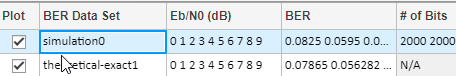
The upper pane of the app is a data set viewer. The data set viewer lists sets of BER data from the current app session along with high level settings and options for showing the data. By default, this data set viewer is empty.
Sets of BER data, generated during the active Bit Error Rate Analysis app session or imported into the session, appear in the data viewer. This figure shows the
simulation0BER data set loaded in the data viewer pane.
The lower pane of the app has tabs labeled Theoretical and Monte Carlo. The tabs correspond to the different methods you can use to generate BER data with the app.
Note
For direct comparisons between theoretical results and simulation results generated when using the Bit Error Rate Analysis app, be sure that your MATLAB function or Simulink® model simulation run from the Monte Carlo tab exactly matches the system defined by the parameters in the Theoretical tab.
For more information, see the Compute Theoretical BERs Using Bit Error Analysis App, Run MATLAB Simulations in Monte Carlo Tab, and Run Simulink Simulations in Monte Carlo Tab sections.
A separate BER Figure window displays the BER data sets that have Plot selected in the data viewer. The BER Figure window does not open until the Bit Error Rate Analysis app has at least one data set to display.
Interaction Between Bit Error Rate Analysis App Components
The components of the app act as one integrated tool.
If you select a data set in the data viewer, the app reconfigures the tabs to reflect the parameters associated with that data set and highlights the corresponding data in the BER Figure window. This feature is useful if the data viewer displays multiple data sets and if you want to recall the meaning and origin of each data set.
If you select data plotted in the BER Figure window, the app reflects the parameters associated with that data in the app panes and highlights the corresponding data set in the data viewer.
Note
You cannot click a data point while the app is generating Monte Carlo simulation results. Before selecting data for more information, you must wait until the app generates all of the data points.
If you configure the Theoretical tab in a way that is already reflected in an existing data set, the app highlights that data set in the data viewer. This feature prevents the app from duplicating its computations and entries in the data viewer but still enables the app to show results that you requested.
If you close the BER Figure window, you can reopen the figure window by selecting BER Figure from the Window menu in the app.
If you select options in the data viewer that affect the BER plot, the BER Figure window automatically reflects your selections. Such options relate to data set names, confidence intervals, curve fitting, and the presence or absence of specific data sets in the BER plot.
Note
If you want to observe the addition of theoretical data to a plot with Monte Carlo simulation data displayed but do not yet have any data sets in the Bit Error Rate Analysis app, you can follow the workflow described in the Use Theoretical Tab in Bit Error Rate Analysis App section.
If you save the BER Figure window using the File menu, the resulting file contains the contents of the window, but not the Bit Error Rate Analysis app data that led to the plot. To save an entire Bit Error Rate Analysis app session, see the Save Bit Error Rate Analysis app Session section.
Compute Theoretical BERs Using Bit Error Analysis App
Section Overview
You can use the Bit Error Rate Analysis app to generate and analyze theoretical BER data. Theoretical data can be useful for comparison with your simulation results. However, closed-form BER expressions exist for only certain kinds of communications systems. For more information, see Analytical Expressions Used in BER Analysis.
To access app capabilities related to theoretical BER data, follow these steps.
Open the Bit Error Rate Analysis app, and select the Theoretical tab.
Set the parameters to reflect the communications system performance that you want to analyze.
Click Plot.
For an example that shows how to generate and analyze theoretical BER data using the Bit Error Rate Analysis app, see the Use Theoretical Tab in Bit Error Rate Analysis App section.
For information about the combinations of parameters available on the Theoretical tab and the underlying functions that perform BER computations, see the Available Sets of Theoretical BER Data section.
Use Theoretical Tab in Bit Error Rate Analysis App
This example shows how to use the app to generate and plot theoretical BER data. In particular, the example compares the performance of different modulation orders for QAM in a communications system that includes an AWGN channel.
Run Theoretical BER Example
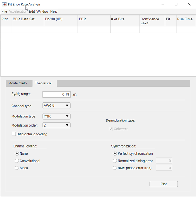
Open the Bit Error Rate Analysis app, and select the Theoretical tab.
Set these parameters to the values specified in this table.
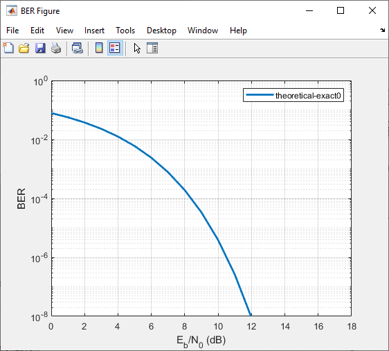
Parameter Value Eb / N0 range 0:18(default)Channel type AWGN(default)Modulation type QAMModulation order 4Click Plot. The app creates an entry in the data viewer and plots the data in the BER Figure window. Although the specified Eb/N0 range is 0:18, the plot includes only BER values that exceed 10-8.
Change the Modulation order parameter to
16, and click Plot. The app creates another entry in the data viewer and plots the new data in the same BER Figure window (not pictured).Change the Modulation order parameter to
64, and click Plot. The app creates another entry in the data viewer and plots the new data in the same BER Figure window.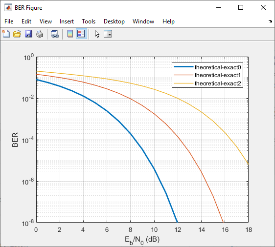
Click one of the curves to view the modulation order for that curve. The app responds to this action by adjusting the parameters in the Theoretical tab to reflect the values that correspond to that curve.
Remove the curve corresponding to 64-QAM from the plot (but not from the data viewer), by clearing Plot for the last entry in the data viewer. To restore the curve for 64-QAM to the plot, in the data viewer, select Plot for that curve.
Available Sets of Theoretical BER Data
The Bit Error Rate Analysis app can generate a large set of theoretical BERs. Parameters in the Theoretical tab enable you to configure the channel type, modulation type and order, error detection and correction channel coding, and synchronization error used when the app computes the theoretical BER. The app adjusts the combination of selectable parameter values based on your choices so that the configuration is always valid or uses a dialog box to inform you of valid parameter values.
The app computes the theoretical BER for these modulation types, assuming Gray ordered binary transmission data. The app uses these BER functions to perform underlying computations and limits the modulation order to practical limits.
berawgn— For AWGN channel systems with no coding and perfect synchronizationberfading— For fading channel systems with no coding and perfect synchronizationbercoding— For systems with channel codingbersync— For systems with BPSK modulation, no coding, and imperfect synchronizationberconfint— For error probability estimate and confidence interval of Monte Carlo simulationberfit— For fitting curves to nonsmooth empirical BER data
To compute the BER for higher modulation orders than permitted in the app, use the BER functions. For more information about specific combinations of parameters, see the reference pages for the BER functions listed in the Bit Error Rate Calculation and Estimation function group of the Test and Measurement category.
Run MATLAB Simulations in Monte Carlo Tab
Section Overview
Using the Monte Carlo tab with the Simulation environment parameter set to MATLAB, you can use the Bit Error Rate Analysis app in conjunction with your own MATLAB communications system simulation functions to generate and analyze BER data. The app calls the simulation specified by the Function name parameter for each specified Eb/N0 value, collects the BER data from the simulation, and creates a plot. The app also enables you to adjust the Eb/N0 range and the stopping criteria for the simulation.
To make your own simulation functions compatible with the app, see the Prepare MATLAB Function for Use in Bit Error Rate Analysis App example on the Bit Error Rate Analysis app reference page.
Use MATLAB Function with Bit Error Rate Analysis App
This example shows how the Bit Error Rate Analysis app can run the
viterbisim
MATLAB simulation.
To run this example, follow these steps.
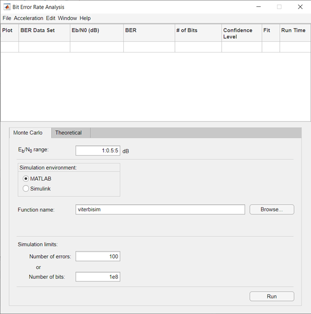
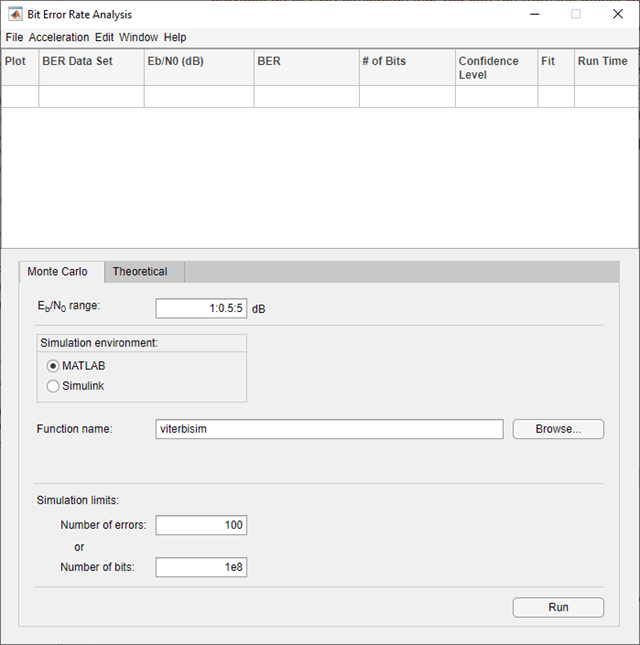
Open the Bit Error Rate Analysis app, and select the Monte Carlo tab.
Set these parameters to the specified values shown in this table.
Parameter Value Eb / N0 range 0:5Simulation environment MATLAB (default) Function name viterbisim(default)Number of Errors 100(default)Number of bits 1e8(default)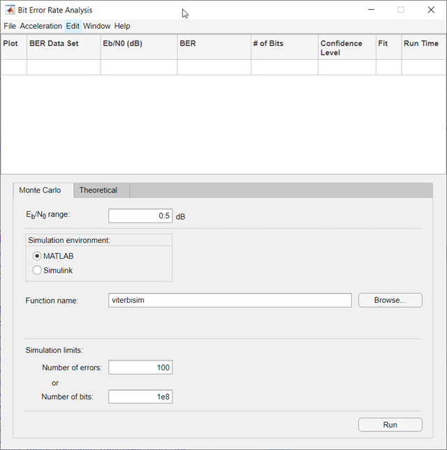
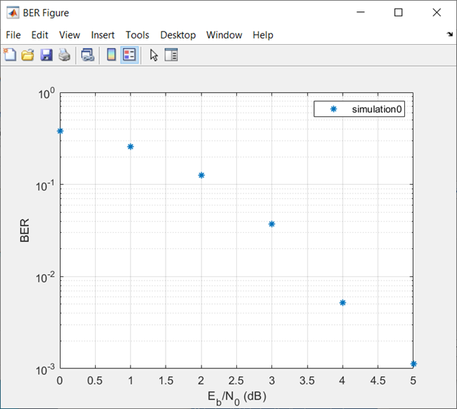
Click Run. The app runs the simulation function once for each specified Eb/N0 value and gathers BER data.
Note
While the Bit Error Rate Analysis app runs the configured simulation, it cannot process certain other tasks, including plotting data from the other tabs of the user interface. However, you can stop the simulation by clicking Stop in the Monte Carlo Simulation dialog box.
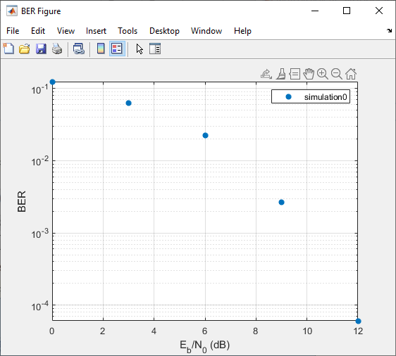
After computing the BER for each of the specified Eb/N0 values, the app creates a listing in the data viewer.
The app also plots the data in the BER Figure window.
Adjust the Eb/N0 range parameter to
[5 5.2 5.3]and the Number of bits parameter to1e5. Click Run to produce a new set of results.The app runs the simulation function using the new Eb/N0 values and computes new BER data. The app then creates another listing in the data viewer.
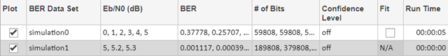
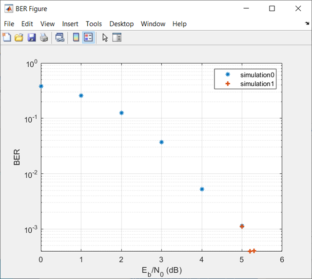
The app also plots the new data set in the BER Figure window, adjusting the horizontal axis to accommodate the new Eb/N0 values.
The BER values for the 5 dB Eb/N0 setting differ between the two sets of data because the number of bits processed by the two simulations was different. If you want the computed BER to converge to a stable value, set the number of bits high enough to ensure that at least 100 bit errors occur. For more information about the criteria used by the Bit Error Rate Analysis app to terminate simulations, see the Assign Function Stopping Criteria section.
Assign Function Stopping Criteria
When you create a MATLAB simulation function for use with the Bit Error Rate Analysis app, control the simulation run duration by setting the target number of errors and maximum number of bits. The simulation stops the current Eb/N0 when either limit is reached. For more information about this requirement, see the Requirements for Using MATLAB Functions with Bit Error Rate Analysis App section.
After you create your function, set the target number of errors and maximum number of bits on the Monte Carlo tab of the app.
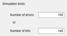
Typically, a Number of errors parameter value of at least
100 produces an accurate error rate. The Number
of bits value prevents the simulation from running too long.
Depending on the
Eb/N0
value and other aspects of the communications system modeled (such as modulation
characteristics and channel conditions), reaching 100 bit errors might not be
realistic. However, if fewer than 100 errors occur because the Number
of bits parameter value is too small, the returned error rate
might be misleading. You can use confidence intervals to gauge the accuracy of
the error rates that your simulation produces. As you increase the confidence
level, the accuracy of the computed error rate decreases.
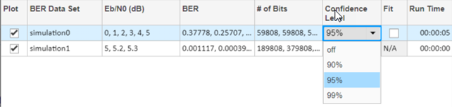
As an example, follow the procedure described in the Use MATLAB Function with Bit Error Rate Analysis App section and set
the Confidence Level parameter value to
95 for each of the two data sets. The
confidence intervals for the second data set are larger than those for the
first data set because the BER values associated with the second data set
are based on only a small number of observed errors.
Note
As long as your function is set up to detect and react to the Stop button in the Bit Error Rate Analysis app, you can use the button to prematurely stop a series of simulations. For more information, see Assign Function Stopping Criteria.
Plot Confidence Intervals
After you run a simulation with the Bit Error Rate Analysis app,
the resulting data set in the data viewer has an active menu in the
Confidence Level column. By default the
Confidence Level value is
off, meaning the simulation data in the BER
Figure window does not show confidence intervals.
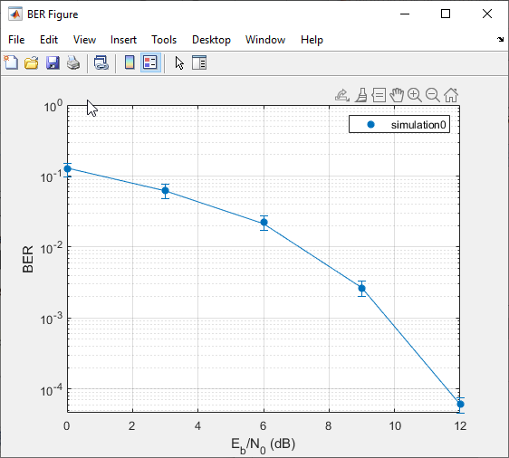
To show confidence intervals in the BER Figure window, set
Confidence Level to 90%,
95%, or 99%.
The plot in the BER Figure window automatically responds the Confidence Level value change. This figure shows a sample plot.
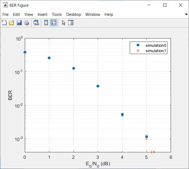
For an example that plots confidence intervals for a Simulink simulation, see the Use Simulink Model with Bit Error Rate Analysis App section.
To find confidence intervals for levels not listed in the Confidence
Level menu, use the berconfint function.
Curve Fit BER Points
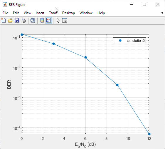
After you run a simulation with the Bit Error Rate Analysis app, the BER Figure window plots individual BER data points. To fit a curve to a data set that contains at least four points, select Fit for that data in the data viewer.

The plot in the BER Figure window automatically responds to this selection. This plot shows a curve fit to a set of BER results.
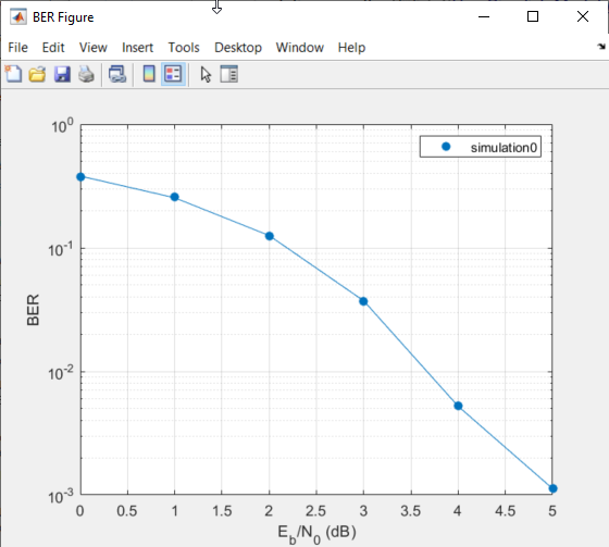
For greater flexibility in the process of fitting a curve to BER data, use the
berfit function.
Requirements for Using MATLAB Functions with Bit Error Rate Analysis App
When you create a MATLAB function for use with the Bit Error Rate Analysis app, ensure the function interacts properly with the user interface. This section describes the inputs, outputs, and basic operation of a function that is compatible with the app.
Input Arguments
The Bit Error Rate Analysis app evaluates your entries in fields of the user interface and passes data to the function as these input arguments (in sequential order).
One value from the Eb/N0 range vector each time the Bit Error Rate Analysis app runs the simulation function
Number of errors value
Number of bits value
Output Arguments
Your simulation function must compute and return these output arguments (in sequential order). The Bit Error Rate Analysis app uses these output arguments when reporting and plotting results.
Bit error rate of the simulation
Number of bits processed when computing the BER
Simulation Function Operation
Your simulation function must perform these tasks:
Simulate the communications system for the Eb/N0 value specified in the first input argument.
Stop simulating when the number of errors or number of processed bits equals or exceeds the corresponding threshold specified in the second or third input argument, respectively.
Detect whether you click Stop in the Bit Error Rate Analysis app to stop the simulation in that case.
Template for Simulation Function
Use this template when adapting your code to work with the Bit Error Rate
Analysis app. You can open the template in an editor by entering
edit bertooltemplate at the MATLAB command prompt. If you develop a simulation function without using
the template, be sure your function satisfies the requirements described in the
Requirements for Using MATLAB Functions with Bit Error Rate Analysis App section.
Note
To use this template, you must insert your own simulation code in the
places marked INSERT YOUR CODE HERE. For a complete
example based on this template, see the Prepare MATLAB Function for Use in Bit Error Rate Analysis App example on the Bit Error Rate Analysis app
reference page.
function [ber,numBits] = bertooltemplateTemp(EbNo,maxNumErrs,maxNumBits,varargin)
%BERTOOLTEMPLATE Template for a BERTool (Bit Error Rate Analysis app) simulation function.
%   This file is a template for a BERTool-compatible simulation function.
%   To use the template, insert your own code in the places marked "INSERT
%   YOUR CODE HERE" and save the result as a file on your MATLAB path. Then
%   use the Monte Carlo pane of BERTool to execute the script.
%
%   [BER, NUMBITS] = YOURFUNCTION(EBNO, MAXNUMERRS, MAXNUMBITS) simulates
%   the error rate performance of a communications system. EBNO is a vector
%   of Eb/No values, MAXNUMERRS is the maximum number of errors to collect
%   before stopping the simulation, and MAXNUMBITS is the maximum number of
%   bits to run before stopping the simulation. BER is the computed bit error
%   rate, and NUMBITS is the actual number of bits run. Simulation can be
%   interrupted only after an Eb/No point is simulated.
%
%   [BER, NUMBITS] = YOURFUNCTION(EBNO, MAXNUMERRS, MAXNUMBITS, BERTOOL)
%   also provides BERTOOL, which is the handle for the BERTool app and can
%   be used to check the app status to interrupt the simulation of an Eb/No
%   point.
%
%   For more information about this template and an example that uses it,
%   see the Communications Toolbox documentation.
%
%   See also BERTOOL and VITERBISIM.

% Copyright 2020 The MathWorks, Inc.

% Initialize variables related to exit criteria.
totErr  = 0; % Number of errors observed
numBits = 0; % Number of bits processed

% --- Set up the simulation parameters. ---
% --- INSERT YOUR CODE HERE.

% Simulate until either the number of errors exceeds maxNumErrs
% or the number of bits processed exceeds maxNumBits.
while((totErr < maxNumErrs) && (numBits < maxNumBits))

    % Check if the user clicked the Stop button of BERTool.
    if isBERToolSimulationStopped(varargin{:})
      break
    end

    % --- Proceed with the simulation.
    % --- Be sure to update totErr and numBits.
    % --- INSERT YOUR CODE HERE.

end % End of loop

% Compute the BER.
ber = totErr/numBits;
About Template for Simulation Function
The simulation function template either satisfies the requirements listed in the Requirements for Using MATLAB Functions with Bit Error Rate Analysis App section or indicates where you need to insert code. In particular, the template:
Has appropriate input and output arguments
Includes a placeholder for code that simulates a system for the given Eb/N0 value
Uses a loop structure to stop simulating when either the number of errors exceeds
maxNumErrsor the number of bits exceedsmaxNumBits, whichever occurs firstNote
Although the
whilestatement of the loop describes the exit criteria, your own code inserted into the section markedProceed with simulationmust compute the number of errors and the number of bits. If you do not perform these computations in your own code, clicking Stop in the Monte Carlo Simulation dialog box is the only way to terminate the loop.Detects when the user clicks Stop in the Monte Carlo Simulation dialog box in each iteration of the loop
Use Simulation Function Template
Follow these steps to update the simulation function template with your own simulation code.
Place the code for setup tasks in the template section marked
Set up parameters. For example, initialize variables such as those containing the modulation alphabet size, filter coefficients, a convolutional coding trellis, or the states of a convolutional interleaver.Place the code for these core simulation tasks in the template section marked
Proceed with simulation. Determine the core simulation tasks, assuming that all setup work has already been performed. For example, core simulation tasks include filtering, error-control coding, modulation and demodulation, and channel modeling.Also in the template section marked
Proceed with simulation, include code that updates the values of thetotErrandnumBitsvariables. ThetotErrvalue represents the number of errors observed so far. ThenumBitsvalue represents the number of bits processed so far. The computations to update these variables depend on how your core simulation tasks work.Note
Updating the numbers of errors and bits is important for ensuring that the loop terminates.
Omit from your simulation code any setup code that initializes
EbNo,maxNumErrs, ormaxNumBitsvariables, because the app passes these quantities to the function as input arguments after evaluating the data entered on the Monte Carlo tab.Adjust your code or the code of the template as necessary to use consistent variable names and meanings. For example, if your original code uses a variable called
ebn0and the function declaration (first line) for the template uses the variable nameEbNo, you must change one of the names so that they match. As another example, if your original code uses SNR instead of Eb/N0 values, you must convert values appropriately.
Compute Error Rate Simulation Sweeps Using Bit Error Rate Analysis App
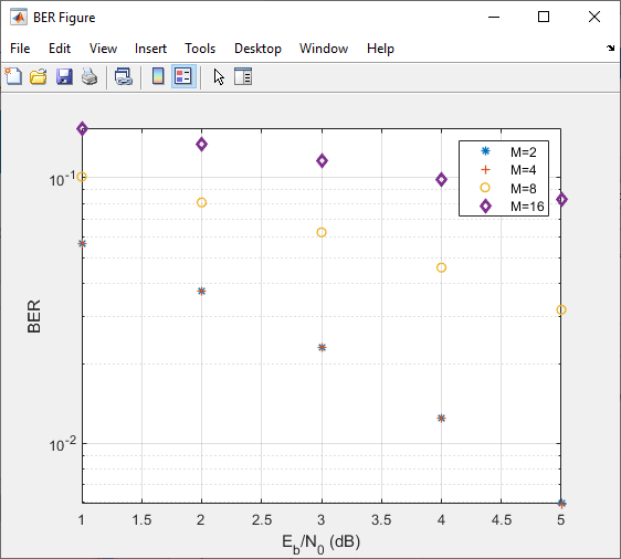
Use the Bit Error Rate Analysis app to compute the BER as a function of . The app analyzes performance with either Monte Carlo simulations of MATLAB® functions and Simulink® models or theoretical closed-form expressions for selected types of communications systems. The code in the mpsksim.m function provides an M-PSK simulation that you can run from the Monte Carlo tab of the app.
Open the Bit Error Rate Analysis app from the Apps tab or by running the bertool function in the MATLAB command window.
On the Monte Carlo tab, set the range parameter to 1:1:5 and the Function name parameter to mpsksim.
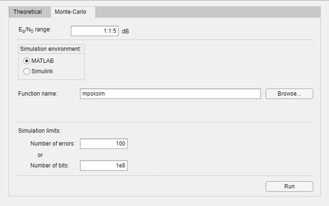
Open the mpsksim function for editing, set M=2, and save the changed file.
Run the mpsksim.m function as configured by clicking Run on the Monte Carlo tab in the app.
After the app simulates the set of points, update the name of the BER data set results by selecting simulation0 in the BER Data Set field and typing M=2 to rename the set of results. The legend on the BER figure updates the label to M=2.


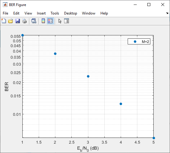
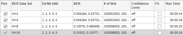
Update the value for M in the mpsksim function, repeating this process for M = 4, 8, and 16. For example, these figures of the Bit Error Rate Analysis app and BER Figure window show results for varying M values.
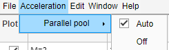
Parallel SNR Sweep Using Bit Error Rate Analysis App
The default configuration for the Monte Carlo processing of the Bit Error Rate Analysis app automatically uses parallel pool processing to process individual points when you have the Parallel Computing Toolbox™ software but for the processing of your simulation code:
Copyright 2020 The MathWorks, Inc.
Run Simulink Simulations in Monte Carlo Tab
Section Overview
You can use the Bit Error Rate Analysis app in conjunction with Simulink models to generate and analyze BER data. The Simulink model simulates the performance of the communications system that you want to study, while the Bit Error Rate Analysis app manages a series of simulations using the model and collects the BER data.
Note
To use Simulink models within the Bit Error Rate Analysis app, you must have the Simulink software.
To access the capabilities of the Bit Error Rate Analysis app
related to Simulink models, open the Monte Carlo tab, and then
set the Simulation environment parameter to
Simulink. If using parallel processing, the output must
be saved to a workspace variable so that the parallel running engine can collect
the results. For example, save the output of the Error Rate Calculation block to a
workspace variable by using a To Workspace (Simulink) block configured to
save the output to the name specified for the BER variable
name and with the Save format set to
Array.
Tip
Select the To Workspace block from the DSP System Toolbox™ / Sinks sublibrary. For more information, see To Workspace Block Configuration for Communications System Simulations.
For details about confidence intervals and curve fitting for simulation data, see the Plot Confidence Intervals and Curve Fit BER Points sections, respectively.
Use Simulink Model with Bit Error Rate Analysis App
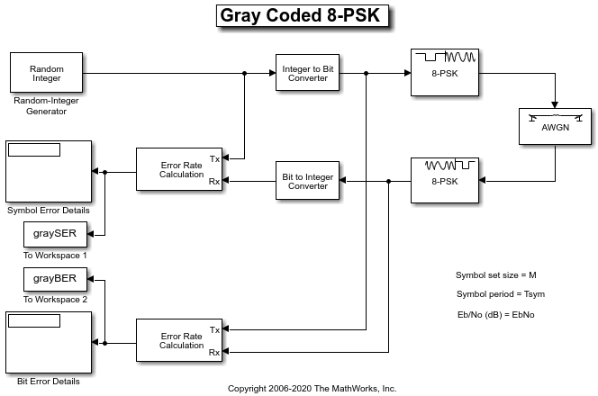
This example shows how the Bit Error Rate Analysis app can manage a
series of simulations of a Simulink model and how you can vary the plot. This figure shows the
commgraycode model.
To run this example, follow these steps.
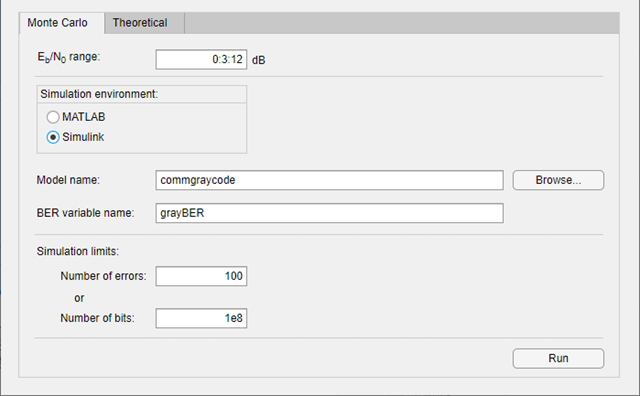
Open the Bit Error Rate Analysis app. On the Monte Carlo tab, enter the Simulink model name and a BER variable name. The default value for the Model name parameter is
commgraycode. the default value for the BER variable name parameter isgrayBER.Click Run.
The Bit Error Rate Analysis app loads the model into memory. The model initializes several variables in the MATLAB workspace. The app runs the simulation model once for each Eb/N0 value, gathers the BER results, and creates a listing for the BER results in the data viewer.

The Bit Error Rate Analysis app plots the data in the BER Figure window.
To fit a curve to the series of points in the BER Figure window, select Fit for the
simulation0data in the data viewer.The Bit Error Rate Analysis app plots the curve.
To indicate a 99% confidence interval around each point in the simulation data, set Confidence Level to
99%in the data viewer.The Bit Error Rate Analysis app displays error bars to represent the confidence intervals.
For another example that uses the Bit Error Rate Analysis app to manage a series of Simulink simulations, see the Prepare Simulink Model for Use with Bit Error Rate Analysis App example on the Bit Error Rate Analysis app reference page.
Assign Model Stopping Criteria
When you create a Simulink model for use with the Bit Error Rate Analysis app, you must set it up so that the simulation ends when it either detects a target number of errors or processes a maximum number of bits, whichever occurs first. For more information about this requirement, see the Requirements for Using Simulink Models with Bit Error Rate Analysis App section.
After creating your Simulink model, set the target number of errors and the maximum number of bits on the Monte Carlo tab of the Bit Error Rate Analysis app.
Typically, a Number of errors parameter value of at least
100 produces an accurate error rate. The Number
of bits value prevents the simulation from running too long,
especially at large
Eb/N0
values. However, if the Number of bits value is so small
that the simulation collects very few errors, the error rate might not be
accurate. You can use confidence intervals to gauge the accuracy of the error
rates that your simulation produces. Larger confidence intervals result in less
accurate computed error rates.
You can also click Stop in the Monte Carlo Simulation dialog box to stop a series of simulations prematurely.
Requirements for Using Simulink Models with Bit Error Rate Analysis App
When you create a Simulink model for use with the Bit Error Rate Analysis app, ensure the model interacts properly with the user interface. This section describes the inputs, outputs, and basic operation of a model that is compatible with the app.
Input Variables
The channel block must use the
EbNovariable rather than a hard-coded value for Eb/N0. For example, to model an AWGN channel, use the AWGN Channel block with the Mode parameter set toSignal to noise ratio (Eb/No)and the Eb/No (dB) parameter set toEbNo.The simulation must stop either when the error count reaches the value of the
maxNumErrsvariable or when the number of processed bits reaches the value of themaxNumBitsvariable, whichever occurs first. You can configure the Error Rate Calculation block in your model to use these criteria to stop the simulation.
Output Variables
The simulation must send the final error rate data to the MATLAB workspace as a variable whose name you enter in the BER variable name parameter in the Bit Error Rate Analysis app. The output error statistics variable must be a three-element vector that lists the BER, the number of bit errors, and the number of processed bits.
The three-element vector format for the output error statistics is supported by the Error Rate Calculation block.
Simulation Model Operation
To avoid using an undefined variable name in blocks of the Simulink model, initialize these variables in the MATLAB workspace by using the preload callback function of the model or by assigning them at the MATLAB command prompt.
EbNo = 0; maxNumErrs = 100; maxNumBits = 1e8;
Tip
Using the preload function callback of the model to initialize the runtime variables enables to you reopen the model in a future MATLAB session with runtime variables preconfigured to run in the app.
The Bit Error Rate Analysis app provides the actual values based on values in the Monte Carlo tab, so the initial values in the model or workspace are not important.
The app assumes the Eb/N0 is used in the channel modeling. If your model uses the AWGN Channel block, and the Mode parameter is not set to
Signal to noise ratio (Eb/No), adapt the block to use the Eb/N0 mode instead. For more information, see the AWGN Channel block reference page.To compute the error rate, use the Error Rate Calculation block with these parameter settings: select Stop simulation, set Target number of errors to
maxNumErrs, and set Maximum number of symbols tomaxNumBits.If your model computes an SER instead of a BER, use the Integer to Bit Converter (Simulink) block to convert symbols to bits.
To send data from the Error Rate Calculation block to the MATLAB workspace, set the Output data parameter to
Port, attach a To Workspace (Simulink) block to the Error Rate Calculation block, and set the Limit data points to last parameter of the To Workspaceblock to1. The Variable name parameter in the To Workspace block must match the value you enter in the BER variable name parameter of the Bit Error Rate Analysis app.Tip
Select the To Workspace block from the DSP System Toolbox / Sinks sublibrary. For more information, see To Workspace Block Configuration for Communications System Simulations.
Frame-based simulations often run faster than sample-based simulations for the same number of bits processed. With a frame-based simulation, because the simulation processes a full frame of data each frame, the number of errors or number of processed bits might exceed the values you enter in the Bit Error Rate Analysis app.
If your model uses a callback function to initialize variables in the MATLAB workspace upon loading the model, before you click Run in the Bit Error Rate Analysis app, make sure that one of these conditions is met:
The model is in memory (whether in a window or not), and the variables are intact.
The model is not currently in memory. In this case, the Bit Error Rate Analysis app loads the model into memory and runs the callback functions.
To close open models without saving any changes made while working with them, clear the models from memory by calling the
bdclose(Simulink) function at the MATLAB command prompt providing the name of the each model individually.When you click Run in the Monte Carlo tab, the app reloads the model.
Manage BER Data
Managing Data in Data Viewer
The data viewer gives you flexibility to rename and delete data sets and to reorder columns in the data viewer.
To rename a data set in the data viewer, double-click its name in the BER Data Set column and type a new name.
To delete a data set from the data viewer, select the data set, then select Edit > Delete.
Note
If the data set originated from the Theoretical tab, the Bit Error Rate Analysis app deletes the data without asking for confirmation. You cannot undo this operation.
Export Bit Error Rate Analysis app Data Set
The Bit Error Rate Analysis app enables you to export individual data sets to the MATLAB workspace or to MAT-files. Exporting data enables you to process the data outside the Bit Error Rate Analysis app. For example, to create customized plots using data from the Bit Error Rate Analysis app, export the app data set to the MATLAB workspace and use any of the plotting commands in MATLAB. To reimport a structure later, see the Import Bit Error Rate Analysis app Data Set section.
To export an individual data set, follow these steps.
In the data viewer, select the data set you want to export.
Select File > Export Data. Set Export to to indicate the format and destination of the data.
Workspace arrays— Export the selected data set to a pair of arrays in the MATLAB workspace. Use this option if you want to access the data in the MATLAB workspace (outside the app) and if you do not need to import the data into the Bit Error Rate Analysis app later.Under Variable names, set Eb/N0 and BER parameters to specify the variable names for the Eb/N0 values and BER values, respectively.
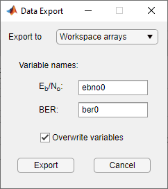
If you want the Bit Error Rate Analysis app to use your chosen variable names even if variables by those names already exist in the workspace, select Overwrite variables.
Workspace structure— Export the selected data set to a structure in the MATLAB workspace. If you export data using this option, you can import the data structure into the Bit Error Rate Analysis app later.Set the Structure name parameter to specify a workspace structure name.

If you want the Bit Error Rate Analysis app to use your chosen variable name even if a variable with that name already exist in the workspace, select Overwrite variables.
MAT-file— Export the selected data set to a structure in a MAT-file. If you export data using this option, you can import a MAT-file data structure into the Bit Error Rate Analysis app later.Set the Structure name in file parameter to specify a MAT-file name. The structure name in the file will also use this name.
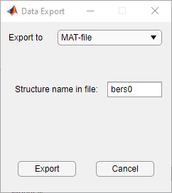
Click OK. If you set Export to to
MAT-file, the Bit Error Rate Analysis app prompts you for the path to the MAT-file that you want to create.
Examine an Exported Structure
This section describes the contents of the structure that the Bit Error
Rate Analysis app exports to the workspace or to a MAT-file. This
table describes the fields of the exported data structure. When you want to
manipulate exported data, the fields that are most relevant are
paramsEvaled and data.
| Field | Description |
|---|---|
params | The parameter values in the Bit Error Rate Analysis app, some of which might be invisible and hence irrelevant for computations |
paramsEvaled | The parameter values evaluated and used by the Bit Error Rate Analysis app when computing the data set |
data | The Eb/N0, BER, and number of bits processed |
dataView | Information about the appearance in the data viewer, which is used by the Bit Error Rate Analysis app when reimporting the data |
cellEditabilities | Indication whether the data viewer has an active Confidence Level or Fit entry, which is used by the Bit Error Rate Analysis app when reimporting the data |
Parameter Fields
The params and paramsEvaled fields are
similar to each other, except that params describes the exact
state of the user interface, whereas paramsEvaled indicates
the values that are actually used for computations. For example, in a
theoretical system with an AWGN channel, params records but
paramsEvaled omits a diversity order parameter. The
diversity order is not used in the computations because it is relevant for only
systems with Rayleigh channels. As another example, if you type
[0:3]+1 in the user interface as the range of
Eb/N0
values, params indicates [0:3]+1, whereas
paramsEvaled indicates 1 2 3 4.
The length and exact contents of paramsEvaled depend on the
data set because only relevant information appears. If the meaning of the
contents of paramsEvaled is not clear upon inspection, one
way to learn more is to reimport the data set into the Bit Error Rate
Analysis app and inspect the parameter values that appear in the user
interface.
Data Field
If your exported workspace variable is called ber0, the
field ber0.data is a cell array that contains the numerical
results in these vectors:
ber0.data{1}lists the Eb/N0 values.ber0.data{2}lists the BER values corresponding to each of the Eb/N0 values.ber0.data{3}indicates, for simulation results, how many bits the Bit Error Rate Analysis app processed when computing each of the corresponding BER values.
Save Bit Error Rate Analysis app Session
The Bit Error Rate Analysis app enables you to save an entire session. This feature is useful if your session contains multiple data sets that you want to return to in a later session. To reimport a saved session, see the Open Previous Bit Error Rate Analysis app Session section.
To save an entire Bit Error Rate Analysis app session, follow these steps.
Select File > Save Session.
When the Bit Error Rate Analysis app prompts you, enter the path to the file that you want to create.
The Bit Error Rate Analysis app saves the data in a MAT file or a binary file that records all data sets currently in the data viewer along with the user interface parameters associated with the data sets.
Note
If your Bit Error Rate Analysis app session requires particular
workspace variables, save those separately in a MAT-file using the
save command in MATLAB.
Import Bit Error Rate Analysis app Data Set
The Bit Error Rate Analysis app enables you to reimport individual data sets that you previously exported to a structure. For more information about exporting data sets from the Bit Error Rate Analysis app, see the Export Bit Error Rate Analysis app Data Set section.
To import an individual data set that you previously exported from the Bit Error Rate Analysis app to a structure, follow these steps.
Select File > Import Data.
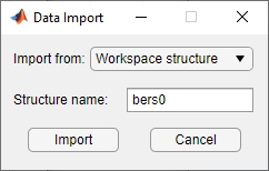
Set the Import from parameter to either
Workspace structureorMAT-file. If you selectWorkspace structure, type the name of the workspace variable in the Structure name parameter.Click OK. If you set Import from to
MAT-file, the Bit Error Rate Analysis app prompts you to select the file that contains the structure you want to import.
After you dismiss the Data Import dialog box (and the file selection dialog box, in the case of a MAT-file), the data viewer shows the newly imported data set and the BER Figure window the corresponding plot.
Open Previous Bit Error Rate Analysis app Session
The Bit Error Rate Analysis app enables you to open previous saved sessions. For more information about exporting data sets from the Bit Error Rate Analysis app, see the Save Bit Error Rate Analysis app Session section.
To replace the data sets in the data viewer with data sets from a previous Bit Error Rate Analysis app session, follow these steps.
Select File > Open Session.
Note
If the Bit Error Rate Analysis app already contains data sets, your are asked whether you want to save the current session. If you answer no and continue with the loading process, the Bit Error Rate Analysis app discards the current session upon opening a new session from the file.
When the Bit Error Rate Analysis app prompts you, enter the path to the file you want to open. It must be a file that you previously created using the Save Session option in the Bit Error Rate Analysis app.
After the Bit Error Rate Analysis app reads the session file, the data viewer shows the data sets from the file.
If the Bit Error Rate Analysis app session requires particular
workspace variables that you saved separately in a MAT-file, you can retrieve
them by using the load function at the
MATLAB command prompt. For example, to load the Bit Error Rate
Analysis app session named
ber_analysis_filename.mat enter this command.
load ber_analysis_filename.mat