再代入したスペクトログラムを使用したリッジの検出と追跡

オオクビワコウモリ ("Eptesicus fuscus") の発する反響定位パルスを 7 マイクロ秒のサンプル レートで測定したデータを含むデータファイルを読み込みます。信号と時間情報を使用して MATLAB® timetable を作成します。この例では、イリノイ大学 Beckman Center の Curtis Condon 氏、Ken White 氏、Al Feng 氏にコウモリのデータの提供および使用許可をいただきました。ご協力に謝意を申し上げます。

load batsignal

t = (0:length(batsignal)-1)*DT;
sg = timetable(seconds(t)',batsignal);

信号アナライザーを開いて、ワークスペース ブラウザーから信号テーブルに timetable をドラッグします。[グリッドの表示] をクリックして、2 つのディスプレイを並べて作成します。各表示を選択し、[表示] タブの [時間-周波数] をクリックしてスペクトログラム表示を追加します。

両方のディスプレイに timetable をドラッグします。

[スペクトログラム] タブを選択します。各ディスプレイについて以下を行います。

• パワーの範囲を -45 dB と -20 dB に設定します。

• 時間分解能を 280 マイクロ秒に指定し、隣接するセグメント間のオーバーラップを 85% に指定します。

• [漏れ] スライダーを使用して、RBW が約 4.5 kHz になるまで漏れを増やします。

右側のディスプレイの [再割り当て] をオンにします。

再割り当てされたスペクトログラムでは、3 つの時間-周波数リッジが明瞭に表示されます。リッジを追跡するために、右側のディスプレイを選択します。[表示] タブの [スクリプトの生成] をクリックして、Spectrogram Script を選択します。スクリプトがエディターで開きます。

% Compute spectrogram

% Generated by MATLAB(R) 9.13 and Signal Processing Toolbox 9.1.
% Generated on: 15-Jun-2022 12:02:38

% Parameters
timeLimits = seconds([0 0.002793]); % seconds
frequencyLimits = [0 71428.57]; % Hz
leakage = 0.9;
timeResolution = 0.00028; % seconds
overlapPercent = 85;
reassignFlag = true;

%%
% Index into signal time region of interest
sg_batsignal_ROI = sg(:,'batsignal');
sg_batsignal_ROI = sg_batsignal_ROI(timerange(timeLimits(1),timeLimits(2),'closed'),1);

% Compute spectral estimate
% Run the function call below without output arguments to plot the results
[P,F,T] = pspectrum(sg_batsignal_ROI, ...
    'spectrogram', ...
    'FrequencyLimits',frequencyLimits, ...
    'Leakage',leakage, ...
    'TimeResolution',timeResolution, ...
    'OverlapPercent',overlapPercent, ...
    'Reassign',reassignFlag);

スクリプトを実行します。再割り当てされたスペクトログラムをプロットします。

mesh(seconds(T),F,P)
xlabel("Time")
ylabel("Frequency")
axis tight
view(2)
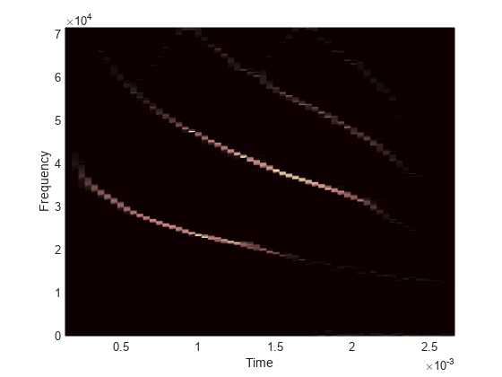
colormap pink

リッジの追跡に関数tfridgeを使用します。

[fridge,~,lridge] = tfridge(P,F,0.01,NumRidges=3,NumFrequencyBins=10);

hold on
plot3(seconds(T),fridge,P(lridge),":",linewidth=3)
hold off

参考

アプリ

• 信号アナライザー

関数

• pspectrum | tfridge | timetable

トピック

• 相関する信号間の遅延の検出
• ウィンドウの漏れを変化させることでトーンを分解する
• 異なるウィンドウを使用した信号スペクトルの計算
• パーシステンス スペクトルを使用した干渉の検出
• 複素包絡線を使用した変調と復調
• 音楽信号からの音声の抽出
• 不等間隔サンプル信号のリサンプリングおよびフィルター処理
• 独自の関数を使用した飽和信号のクリップ除去
• 振動信号の包絡線スペクトルの計算
• クジラの歌からの関心領域の抽出
• 信号アナライザー アプリの使用
• サンプル レートおよびその他の時間情報の編集
• 信号アナライザーでサポートされるデータ型
• 信号アナライザーでのスペクトル計算
• 信号アナライザーのパーシステンス スペクトル
• 信号アナライザーでのスペクトログラム計算
• 信号アナライザーでのスカログラム計算
• 信号アナライザーのキーボード ショートカット
• 信号アナライザーのヒントと制限