geoplot

Plot points, lines, and polygons on map

Since R2022a

Syntax

geoplot(GT)

geoplot(shape)

geoplot(___,LineSpec)

geoplot(lat,lon)

geoplot(lat,lon,LineSpec)

geoplot(lat1,lon1,...,latN,lonN)

geoplot(lat1,lon1,LineSpec1,...,latN,lonN,LineSpecN)

geoplot(tbl,latvar,lonvar)

geoplot(___,Name=Value)

geoplot(ax,___)

h = geoplot(___)

Description

Mapping Toolbox™ extends the functionality of the geoplot (MATLAB^®) function. It adds support for displaying points, lines, and polygons with coordinates in any supported geographic or projected coordinate reference system (CRS). Depending on the type of axes, the function displays data into different map projections.

• Geographic axes — A Web Mercator projection

• Map axes — The projection specified by the ProjectedCRS property of the map axes

If you do not have Mapping Toolbox installed, then see geoplot.

Geospatial Table and Shape Data

geoplot(GT) plots the point, line, or polygon shape objects within the Shape variable of the geospatial table GT. If the current axes is not a geographic or map axes, or if there is no current axes, then the function plots the line in a new geographic axes.

geoplot(shape) plots the point, line, or polygon shape objects in shape.

geoplot(___,LineSpec) sets the style, marker symbol, and color for the plotted shapes. You can use the LineSpec argument with either the GT or shape argument.

Numeric Vector Data

geoplot(lat,lon) plots a line with vertices at the latitudes and longitudes in lat and lon, respectively.

geoplot(lat,lon,LineSpec) sets the style, marker symbol, and color for the line.

geoplot(lat1,lon1,...,latN,lonN) plots multiple pairs of latitude and longitude coordinates on the same set of axes.

geoplot(lat1,lon1,LineSpec1,...,latN,lonN,LineSpecN) assigns specific line styles, markers, and colors to each latitude-longitude pair.

Numeric Table Data

geoplot(tbl,latvar,lonvar) plots the variables latvar and lonvar from the table tbl. To plot one data set, specify one variable for latvar and one variable for lonvar. To plot multiple data sets, specify multiple variables for latvar, lonvar, or both. If both arguments specify multiple variables, they must specify the same number of variables. (Since R2022b)

Additional Options

geoplot(___,Name=Value) specifies options for the plot using one or more name-value arguments, in addition to any combination of input arguments from the previous syntaxes.

geoplot(ax,___) plots in the geographic axes or map axes specified by ax.

h = geoplot(___) returns a Point, Line, or Polygon object. The type of object depends on the type of input. Use h to modify the properties of the plot object.

Examples

Plot Shapes from Geospatial Table

Import a shapefile containing road data for Concord, MA, into the workspace as a geospatial table. The table represents roads using line shapes in projected coordinates.

GT = readgeotable("concord_roads.shp");
GT.Shape

Display the line shapes by passing the table to the geoplot function.

figure
geoplot(GT)

Change the basemap and add a title.

geobasemap streets
title("Road Network Over Streets Basemap")

Plot from Geospatial Table Using Custom Colors

One way to plot data from a geospatial table and customize the colors is to set the ColorVariable property. You can set this property by using a name-value argument when you call the geoplot function, or you can set it on the plot object later.

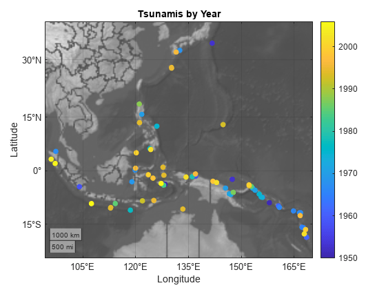
Read a shapefile containing tsunami events into the workspace as a geospatial table. The table represents the tsunami events using point shapes in geographic coordinates.

GT = readgeotable("tsunamis.shp",CoordinateSystemType="geographic");

Create a subtable containing events for a region surrounding Southeast Asia.

bbox = geopolyshape([-25 35 35 -25 -25],[90 90 170 170 90]);
inpoly = isinterior(bbox,GT.Shape);
GT2 = GT(inpoly,:);

Display the point shapes within the table. Vary the marker colors by specifying the ColorVariable name-value argument as a table variable. Return the Point object as h, so you can change the ColorVariable property later.

figure
h = geoplot(GT2,ColorVariable="Year",MarkerSize=20);

Change the basemap, add a colorbar, and add a title.

geobasemap grayterrain
colorbar
title("Tsunamis by Year")

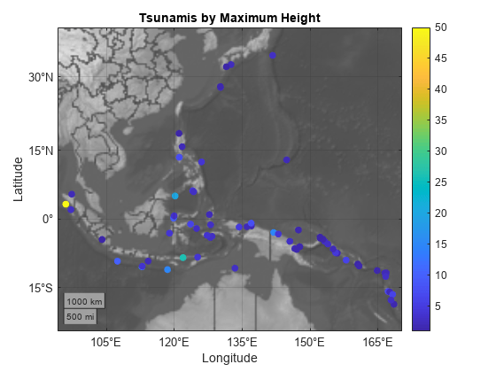
Change the marker colors again by setting the ColorVariable property to a different table variable.

h.ColorVariable = "Max_Height";
title("Tsunamis by Maximum Height")

Plot Shapes in Geographic Coordinates

Read a shapefile containing world cities into the workspace as a geospatial table. The table represents the cities using point shapes in geographic coordinates.

GT = readgeotable("worldcities.shp");
shape = GT.Shape

shape = 
  318×1 geopointshape array with properties:

               NumPoints: [318×1 double]
                Latitude: [318×1 double]
               Longitude: [318×1 double]
                Geometry: "point"
    CoordinateSystemType: "geographic"
           GeographicCRS: [1×1 geocrs]

Clip the shapes to a region containing part of Europe.

clipped = geoclip(shape,[30 60],[-20 35]);

Display the shapes using red plus sign markers over a topographic basemap.

figure
geoplot(clipped,"r+")
geobasemap topographic
title("Cities Over Topographic Basemap")

Plot Shapes in Projected Coordinates

Read hydrography data into the workspace as a geospatial table. The table represents the data using polygon shapes in projected coordinates. Extract the polygon shape for a pond.

GT = readgeotable("concord_hydro_area.shp");
shape = GT.Shape(14)

shape = 
  mappolyshape with properties:

              NumRegions: 1
                NumHoles: 3
                Geometry: "polygon"
    CoordinateSystemType: "planar"
            ProjectedCRS: [1x1 projcrs]

To plot shapes in projected coordinates using the geoplot function, the ProjectedCRS property of the shape must not be empty. View the contents of the ProjectedCRS property.

shape.ProjectedCRS

ans = 
  projcrs with properties:

                    Name: "NAD83 / Massachusetts Mainland"
           GeographicCRS: [1x1 geocrs]
        ProjectionMethod: "Lambert Conic Conformal (2SP)"
              LengthUnit: "meter"
    ProjectionParameters: [1x1 map.crs.ProjectionParameters]

Create a new map that uses the same projected CRS as the pond polygon. Then, display the pond polygon.

figure
newmap(shape.ProjectedCRS)
geoplot(shape)

Title the map using the name of the projected CRS.

title(shape.ProjectedCRS.Name)

Plot Shapes Using Custom Colors

Read a shapefile of US states into the workspace as a geospatial table. The table represents the states using polygon shapes in geographic coordinates.

GT = readgeotable("usastatehi.shp");
shape = GT.Shape;

Clip the shapes to a region containing the conterminous US.

clipped = geoclip(shape,[17 56],[-127 -65]);

Create a new map that uses a North America Albers Equal Area Conic projection. Then, display the shapes. Vary the colors by using the ColorData name-value argument.

figure
proj = projcrs(102008,Authority="ESRI");
newmap(proj)

c = 1:length(clipped);
geoplot(clipped,ColorData=c)

Add a title.

title("Conterminous US")

Plot Points and Lines from Numeric Vector Data

Load a MAT file containing the coordinates of global coastlines into the workspace. The variables within the MAT file, coastlat and coastlon, specify numeric latitude and longitude coordinates, respectively. Display the coordinates using a blue line over a topographic basemap.

load coastlines
figure
geoplot(coastlat,coastlon,"b")
geobasemap topographic

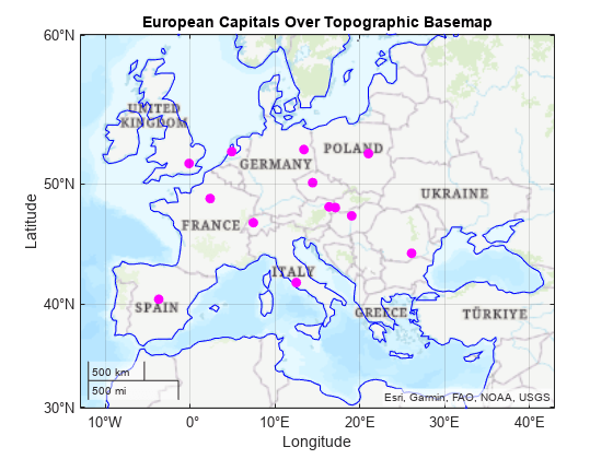
Read the geographic coordinates of European capitals into the workspace. Display the capitals using magenta circle markers on the same map.

[lat,lon] = readvars("european_capitals.txt");
hold on
geoplot(lat,lon,"om",MarkerFaceColor="m")
title("European Capitals Over Topographic Basemap")

Center the map over Europe by changing its limits.

geolimits([30 60],[-13 43])

Plot Point, Line, and Polygon Shapes on Same Axes

Import several shapefiles into the workspace as geospatial tables.

• landareas.shp contains world land areas. The table represents the areas using polygon shapes in geographic coordinates (geopolyshape objects).

• worldrivers.shp contains world rivers. The table represents the rivers using line shapes in geographic coordinates (geolineshape objects).

• worldcities.shp contains world cities. The table represents the cities using point shapes in geographic coordinates (geopointshape objects).

land = readgeotable("landareas.shp");
rivers = readgeotable("worldrivers.shp");
cities = readgeotable("worldcities.shp");

Set up a new map. By default, map axes use an Equal Earth map projection. Then, display each set of shapes using separate calls to the geoplot function. Different shapes support different name-value arguments.

• Display the land areas using green polygons.

• Display the rivers using blue lines.

• Display the cities using black points.

figure
newmap
hold on

geoplot(land,FaceColor=[0.7 0.9 0.5],EdgeColor=[0.7 0.9 0.5])
geoplot(rivers,Color=[0 0.4470 0.7410])
geoplot(cities,"k")

Add a title.

title("World Land Areas, Rivers, and Cities")

Specify Geographic Axes

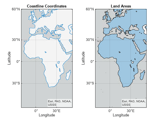
Create multiple geographic axes in a single figure by using a tiled chart layout.

Create a 1-by-2 tiled chart layout.

t = tiledlayout(1,2);

Load a MAT file containing the coordinates of global coastlines into the workspace. The variables within the MAT file, coastlat and coastlon, specify numeric latitude and longitude coordinates, respectively.

load coastlines

Place a geographic axes in the first tile. Plot the coordinates as a line on the axes.

gx1 = geoaxes(t);
geoplot(gx1,coastlat,coastlon)
title(gx1,"Coastline Coordinates")

Read a shapefile containing world land areas into the workspace as a geospatial table. The table represents the land areas using polygon shapes in geographic coordinates.

GT = readgeotable("landareas.shp");

Place a new geographic axes in the second tile. Plot the land areas as a polygon on the new axes.

gx2 = geoaxes(t);
gx2.Layout.Tile = 2;
geoplot(gx2,GT)
title(gx2,"Land Areas")

Zoom both axes to a region containing Africa.

latlim = [-55 60];
lonlim = [-21 53];
geolimits(gx1,latlim,lonlim)
geolimits(gx2,latlim,lonlim)

Modify Point, Line, or Polygon After Creation

Import several shapefiles into the workspace as geospatial tables.

• landareas.shp contains world land areas. The table represents the areas using polygon shapes in geographic coordinates (geopolyshape objects).

• worldrivers.shp contains world rivers. The table represents the rivers using line shapes in geographic coordinates (geolineshape objects).

• worldcities.shp contains world cities. The table represents the cities using point shapes in geographic coordinates (geopointshape objects).

land = readgeotable("landareas.shp");
rivers = readgeotable("worldrivers.shp");
cities = readgeotable("worldcities.shp");

Display each set of shapes by using separate calls to the geoplot function.

• Display the land areas and return the polygon in h1. The polygon in h1 represents multiple polygon shapes in land.

• Display the rivers and return the line in h2. The line in h2 represents multiple line shapes in rivers.

• Display the cities and return the point in h3. The point in h3 represents multiple point shapes in cities.

figure
h1 = geoplot(land);
hold on
h2 = geoplot(rivers);
h3 = geoplot(cities);

Change the geographic limits of the map, add a title, and remove the basemap.

geolimits([-72 85],[-180 180])
title("World Land Areas, Rivers, and Cities")
geobasemap none

Update properties of the polygon, point, and line objects. Each object supports different properties.

• Change the fill and outline colors of the polygons to green.

• Change the color of the lines to blue.

• Change the color of the markers to black.

h1.FaceColor = [0.7 0.9 0.5];
h1.EdgeColor = [0.7 0.9 0.5];
h2.Color = [0 0.4470 0.7410];
h3.MarkerEdgeColor = "k";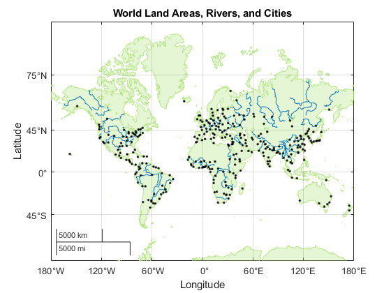

Input Arguments

GT — Geospatial table

geospatial table

Geospatial table. A geospatial table is a table or timetable object with a Shape variable that contains point, line, or polygon shapes. For more information about geospatial tables, see Create Geospatial Tables.

The Shape variable of the table must contain only one type of shape.

The ProjectedCRS property of mappointshape, maplineshape, and mappolyshape objects within the Shape variable must not be empty.

If the GeographicCRS property of a geopointshape, geolineshape, or geopolyshape object within the Shape variable is empty, then the function assumes the geographic CRS based on the type of axes:

• Geographic axes — The WGS84 coordinate reference system.

• Map axes — The geographic CRS specified by the ProjectedCRS property of the map axes. To find the geographic CRS, access the projected CRS in the ProjectedCRS property. Then, access the GeographicCRS property of the projected CRS. For example, to find the geographic CRS for a map axes mx, query mx.ProjectedCRS.GeographicCRS.

shape — Point, line, or polygon shapes

vector of geopointshape objects | vector of geolineshape objects | vector of geopolyshape objects | vector of mappointshape objects | vector of maplineshape objects | vector of mappolyshape objects

Point, line, or polygon shapes, specified as one of these options:

• A vector of geopointshape objects — Point shapes in geographic coordinates

• A vector of geolineshape objects — Line shapes in geographic coordinates

• A vector of geopolyshape objects — Polygon shapes in geographic coordinates

• A vector of mappointshape objects — Point shapes in projected coordinates

• A vector of maplineshape objects — Line shapes in projected coordinates

• A vector of mappolyshape objects — Polygon shapes in projected coordinates

You can also specify this argument as a scalar point, line, or polygon shape.

The ProjectedCRS property of mappointshape, maplineshape, and mappolyshape objects must not be empty.

If the GeographicCRS property of a geopointshape, geolineshape, or geopolyshape object within the Shape variable is empty, then the function assumes the geographic CRS based on the type of axes:

• Geographic axes — The WGS84 coordinate reference system.

• Map axes — The geographic CRS specified by the ProjectedCRS property of the map axes. To find the geographic CRS, access the projected CRS in the ProjectedCRS property. Then, access the GeographicCRS property of the projected CRS. For example, to find the geographic CRS for a map axes mx, query mx.ProjectedCRS.GeographicCRS.

lat — Latitude coordinates in degrees

vector

Latitude coordinates in degrees, specified as a vector. The vector can contain NaN values.

Depending on the type of axes, the geoplot function references numeric coordinates to different geographic CRSs.

• Geographic axes — The WGS84 coordinate reference system. To plot points or lines with coordinates in a different CRS, use the coordinates to create a geopointshape or geolineshape object and set its GeographicCRS property. Then, pass the object you created to the geoplot function.

• Map axes — The geographic CRS specified by the ProjectedCRS property of the map axes. To find the geographic CRS, access the projected CRS in the ProjectedCRS property. Then, access the GeographicCRS property of the projected CRS. For example, to find the geographic CRS for a map axes mx, query mx.ProjectedCRS.GeographicCRS.

lat must be the same size as lon.

Example: [43.0327 38.8921 44.0435]

Data Types: single | double

lon — Longitude coordinates in degrees

vector

Longitude coordinates in degrees, specified as a vector. The vector can contain NaN values.

Depending on the type of axes, the geoplot function references numeric coordinates to different geographic CRSs.

• Geographic axes — The WGS84 coordinate reference system. To plot points or lines with coordinates in a different CRS, use the coordinates to create a geopointshape or geolineshape object and set its GeographicCRS property. Then, pass the object you created to the geoplot function.

• Map axes — The geographic CRS specified by the ProjectedCRS property of the map axes. To find the geographic CRS, access the projected CRS in the ProjectedCRS property. Then, access the GeographicCRS property of the projected CRS. For example, to find the geographic CRS for a map axes mx, query mx.ProjectedCRS.GeographicCRS.

lon must be the same size as lat.

Example: [-107.5556 -77.0269 -72.5565]

Data Types: single | double

LineSpec — Line style, marker, and color

character vector | string scalar

Line style, marker, and color, specified as a character vector or string scalar containing symbols. You can specify the symbols in any order. Different types of input support different characteristics (line, marker style, and color).

Type of Input	Supported Characteristics	Example
GT or shape contains geopointshape or mappointshape objects	Marker and color	'ro' specifies red circle markers
GT or shape contains geolineshape or maplineshape objects	Line style and color	'r--' specifies red dashed lines
GT or shape contains geopolyshape or mappolyshape objects	Line style and color	'r--' specifies red dashed lines
lat and lon contain numeric data	Line style, marker, and color	'--or' specifies red dashed lines with circle markers

You do not need to specify all supported characteristics. For example, if you plot a line from numeric data and specify only the marker, then the plot shows only the marker and no line.

Line Style	Description	Resulting Line
"-"	Solid line
"--"	Dashed line
":"	Dotted line
"-."	Dash-dotted line

Marker	Description	Resulting Marker
"o"	Circle
"+"	Plus sign
"*"	Asterisk
"."	Point
"x"	Cross
"_"	Horizontal line
"|"	Vertical line
"square"	Square
"diamond"	Diamond
"^"	Upward-pointing triangle
"v"	Downward-pointing triangle
">"	Right-pointing triangle
"<"	Left-pointing triangle
"pentagram"	Pentagram
"hexagram"	Hexagram

Color Name	Short Name	RGB Triplet	Appearance
"red"	"r"	[1 0 0]
"green"	"g"	[0 1 0]
"blue"	"b"	[0 0 1]
"cyan"	"c"	[0 1 1]
"magenta"	"m"	[1 0 1]
"yellow"	"y"	[1 1 0]
"black"	"k"	[0 0 0]
"white"	"w"	[1 1 1]

tbl — Source table

table | timetable

Source table containing the data to plot, specified as a table or a timetable.

latvar — Table variables containing latitude coordinates

string array | character vector | cell array | pattern | numeric scalar or vector | logical vector | vartype()

Table variables containing the latitude coordinates, specified using one of the indexing schemes from the table.

Indexing Scheme	Examples
Variable names: A string, character vector, or cell array. A pattern object.	"A" or 'A' — A variable named A ["A","B"] or {'A','B'} — Two variables named A and B "Var"+digitsPattern(1) — Variables named "Var" followed by a single digit
Variable index: An index number that refers to the location of a variable in the table. A vector of numbers. A logical vector. Typically, this vector is the same length as the number of variables, but you can omit trailing 0 or false values.	3 — The third variable from the table [2 3] — The second and third variables from the table [false false true] — The third variable
Variable type: A vartype subscript that selects variables of a specified type.	vartype("categorical") — All the variables containing categorical values

Regardless of the variable name, the axis label on the plot is always Latitude.

The variables you specify must contain numeric data of type single or double. The data must be in the range (–90, 90).

If latvar and lonvar both specify multiple variables, the number of variables must be the same.

Example: geoplot(tbl,["lat1","lat2"],"lon") specifies the table variables named lat1 and lat2 for the latitude coordinates.

Example: geoplot(tbl,2,"lon") specifies the second variable for the latitude coordinates.

Example: geoplot(tbl,vartype("numeric"),"lon") specifies all numeric variables for the latitude coordinates.

lonvar — Table variables containing longitude coordinates

string array | character vector | cell array | pattern | numeric scalar or vector | logical vector | vartype()

Table variables containing the longitude coordinates, specified using one of the indexing schemes from the table.

Indexing Scheme	Examples
Variable names: A string, character vector, or cell array. A pattern object.	"A" or 'A' — A variable named A ["A","B"] or {'A','B'} — Two variables named A and B "Var"+digitsPattern(1) — Variables named "Var" followed by a single digit
Variable index: An index number that refers to the location of a variable in the table. A vector of numbers. A logical vector. Typically, this vector is the same length as the number of variables, but you can omit trailing 0 or false values.	3 — The third variable from the table [2 3] — The second and third variables from the table [false false true] — The third variable
Variable type: A vartype subscript that selects variables of a specified type.	vartype("categorical") — All the variables containing categorical values

Regardless of the variable name, the axis label on the plot is always Longitude.

The variables you specify must contain numeric data of type single or double.

If latvar and lonvar both specify multiple variables, the number of variables must be the same.

Example: geoplot(tbl,"lat",["lon1","lon2"]) specifies the table variables named lon1 and lon2 for the longitude coordinates.

Example: geoplot(tbl,"lat",2) specifies the second variable for the longitude coordinates.

Example: geoplot(tbl,"lat",vartype("numeric")) specifies all numeric variables for the longitude coordinates.

ax — Target axes

GeographicAxes object | MapAxes object

Target axes, specified as a GeographicAxes object¹ or MapAxes object. If you do not specify this argument, then the geoplot function plots into the current axes, provided that the current axes is a geographic or map axes object.

Name-Value Arguments

Specify optional pairs of arguments as Name1=Value1,...,NameN=ValueN, where Name is the argument name and Value is the corresponding value. Name-value arguments must appear after other arguments, but the order of the pairs does not matter.

Example: geoplot(47,-122,Marker="*",Color="m") displays a magenta star marker at the specified latitude and longitude.

Specify properties for the plot by using name-value arguments. The supported name-value arguments depend on the type of input.

Type of Input	Supported Name-Value Arguments
GT or shape contains geopointshape or mappointshape objects	See Point Properties
GT or shape contains geolineshape or maplineshape objects	See Line Properties
GT or shape contains geopolyshape or mappolyshape objects	See Polygon Properties
lat and lon contain numeric data	See Line Properties

Output Arguments

h — Plot object

geographic Point object | geographic chart Line object | geographic Polygon object | column vector of chart Line objects

Plot object. The value of h depends on the type of input you pass to the geoplot function.

Type of Input	Value of h
GT or shape contains geopointshape or mappointshape objects	A geographic Point object. A Point object can represent multiple geopointshape or mappointshape objects. For more information about Point objects, see Point Properties.
GT or shape contains geolineshape or maplineshape objects	A geographic chart Line object. A Line object can represent multiple geolineshape or maplineshape objects. For more information about Line objects, see Line Properties.
GT or shape contains geopolyshape or mappolyshape objects	A geographic Polygon object. A Polygon object can represent multiple geopolyshape or mappolyshape objects. For more information about Polygon objects, see Polygon Properties.
lat and lon contain numeric data	A column vector of chart Line objects. Each object corresponds to a vector of latitude-longitude pairs. For more information about Line objects, see Line Properties.

Version History

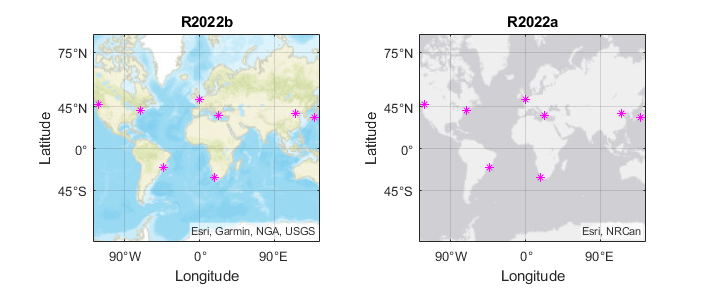
Introduced in R2022a

R2022b: Pass tables containing numeric coordinates directly to geoplot

Create a plot by passing a table containing numeric coordinate data to the geoplot function followed by the coordinate variables you want to plot.

R2022b: Adding new plots to geographic axes does not reset basemap

When you plot into geographic axes by using functions such as geoplot or geoscatter, MATLAB does not reset the basemap. In R2022a and earlier releases, the basemap resets when you add new plots.

As a result, you can specify a basemap and then visualize data without using the hold function between commands. For example, this code creates a map using the streets basemap. Then it displays a plot over the basemap. In R2022b, the basemap does not reset. In R2022a and earlier releases, the basemap resets to the default streets-light.

lat = [35 -22 51 39 37 42 47 -33];
lon = [139 -43 0 116 23 -71 -122 18];
 
figure
geobasemap streets
geoplot(lat,lon,"m*")

This change does not affect existing code that sets the hold state to "on" between commands.

To reset the basemap when you add a new plot, use the cla reset syntax of the cla function before you create the plot. For example, to update the preceding code, use cla reset between the calls to geobasemap and geoplot.

lat = [35 -22 51 39 37 42 47 -33];
lon = [139 -43 0 116 23 -71 -122 18];
 
figure
geobasemap streets
cla reset
geoplot(lat,lon,"m*")

Alternatively, you can change the basemap to the default streets-light by using the geobasemap function. For more information about changing the basemap of geographic axes, see Access Basemaps for Geographic Axes and Charts.