idnlhw

Hammerstein-Wiener Model

Description

An idnlhw model represents a Hammerstein-Wiener model, which is a nonlinear model that is composed of a linear dynamic element and nonlinear functions of the inputs and outputs of the linear system. These nonlinear functions are known as nonlinearity estimators, or more generally as mapping objects.

The following figure illustrates the structure of the Hammerstein-Wiener model.

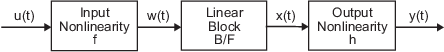
The software computes the Hammerstein-Wiener model output y in three stages:

1. It uses the input nonlinearity f to transform the input vector u(t) into the intermediate variable w(t)

   The input nonlinearity is a static (memoryless) function, where the value of the output a given time t depends only on the input value at time t.

   You can configure the input nonlinearity as a sigmoid network, wavelet network, saturation, dead zone, piecewise linear function, one-dimensional polynomial, or custom network. You can also remove the input nonlinearity by applying a unit gain.

2. It uses w(t) as the input to the dynamic linear block, which you configure as the transfer function B/F. The output of the linear block is x(t).

3. It transforms x(t) using the output nonlinearity h. The output of the block is y(t).

   Similar to the input nonlinearity, the output nonlinearity is a static function. You can configure the output nonlinearity in the same way as the input nonlinearity. In addition to the input nonlinearity options, you also configure the output nonlinearity as a Gaussian process.

The resulting Hammerstein-Wiener models are idnlhw objects that store all model data, including the parameters of the input and output nonlinearities and the coefficients of the transfer function. For more information about these objects, see Nonlinear Model Structures.

For more detail on Hammerstein-Wiener models, including the computation stages, see What Are Hammerstein-Wiener Models?.

For idnlhw object properties, see Properties.

Creation

You can obtain an idnlhw object in one of two ways.

• Use the nlhw command to both construct an idnlhw object and estimate the model parameters.

  sys = nlhw(Data,Orders,InputNL,OutputNL)

• Use the idnlhw constructor to create the Hammerstein-Wiener model and then estimate the model parameters using nlhw or pem. This syntax is useful when you need to customize the model structure, such as when you want to fix certain coefficients to their initial values, before performing an estimation.

  sys = idnlhw(Orders,InputNL,OutputNL))

Syntax

sys = idnlhw(Orders)

sys = idnlhw(Orders,InputNonlinearity,OutputNonlinearity)

sys = idnlhw(LinModel)

sys = idnlhw(LinModel,InputNonlinearity,OutputNonlinearity)

sys = idnlhw(___,Name,Value)

Description

Specify Model Directly

sys = idnlhw(Orders) creates a Hammerstein-Wiener model with the specified orders, and using piecewise linear functions as input and output nonlinearities.

sys = idnlhw(Orders,InputNonlinearity,OutputNonlinearity) uses InputNonlinearity and OutputNonlinearity as the input and output nonlinearity estimators, respectively.

Initialize Model Values Using Linear Model

sys = idnlhw(LinModel) uses a linear model LinModel to specify the model orders and default piecewise linear functions for the input and output nonlinearity estimators.

sys = idnlhw(LinModel,InputNonlinearity,OutputNonlinearity) specifies input and output nonlinearity estimators for the model.

Specify Model Properties

sys = idnlhw(___,Name,Value) specifies additional attributes of the idnlhw model structure using one or more Name,Value arguments. You can use this syntax with any of the previous input argument combinations.

Input Arguments

Orders — Order and delays of the linear subsystem transfer function

[nb nf nk] vector of positive integers | [nb nf nk] vector of matrices

Order and delays of the linear subsystem transfer function, specified as a [nb nf nk] vector.

Dimensions of Orders:

• For a SISO transfer function, Orders is a vector with 3 positive integers.

  nb is the number of zeros plus 1, nf is the number of poles, and nk is the input delay.

• For a MIMO transfer function with nu inputs and ny outputs, Orders is a vector of matrices.

  nb, nf, and nk are ny-by-nu matrices whose i-jth entry specifies the orders and delay of the transfer function from the jth input to the ith output.

LinModel — Discrete time linear model

idpoly model | idss model | idtf model

Discrete-time linear model used to specify the linear subsystem, specified as one of the following:

• Input-output polynomial model of Output-Error (OE) structure (idpoly)

• State-space model (idss)

• Transfer function model (idtf)

Typically, you estimate the model using oe, n4sid, or tfest.

Properties

nb, nf, nk — Model orders and delays

[nb nf nk] vector of positive integers | [nb nf nk] vector of matrices

Model orders and delays of the linear subsystem transfer function, where nb is the number of zeros plus 1, nf is the number of poles, and nk is the input delay.

For a MIMO transfer function with nu inputs and ny outputs, nb, nf, and nk are ny-by-nu matrices whose i-jth entry specifies the orders and delay of the transfer function from the jth input to the ith output.

B — Linear block numerator

cell array

Linear block numerator polynomial B, specified as a cell array of ny-by-nu elements, where ny is the number of outputs and nu is the number of inputs. An element B{i,j} is a row vector representing the numerator polynomial for the jth input to ith output transfer function. The element contains nk leading zeros, where nk is the number of input delays.

F — Linear block denominator

cell array

Linear block denominator polynomial F, specified as a cell array of ny-by-nu elements, where ny is the number of outputs and nu is the number of inputs. An element F{i,j} is a row vector representing the denominator polynomial for the jth input to ith output transfer function.

Bfree — Option to fix or free parameters of B

logical matrix

Option to fix or free the parameters of the B polynomial, specified as a logical matrix of ny-by-nu elements, where ny is the number of outputs and nu is the number of inputs. An element Bfree(i,j) is a row vector representing the numerator polynomial for the jth input to ith output transfer function. Bfree(i,j) = false causes the numerator of the linear transfer function between the input j and output i to be fixed to B(i,j)}. The software honors the Bfree specification only if the B polynomial contains finite values.

Ffree — Option to fix or free the parameters of F

logical matrix

Option to fix or free the parameters of the F polynomial, specified as a logical matrix of ny-by-nu elements, where ny is the number of outputs and nu is the number of inputs. An element Ffree(i,j) is a row vector representing the numerator polynomial for the jth input to ith output transfer function. Ffree(i,j) = false causes the numerator of the linear transfer function between the input j and output i to be fixed to F(i,j). The software honors the Ffree specification only if the F polynomial contains finite values.

InputNonlinearity — Input nonlinearity estimator

idPiecewiseLinear (default) | 'idSigmoidNetwork' | 'idWaveletNetwork' | 'idSaturation' | idDeadZone | 'idPolynomial1D' | 'idUnitGain' | 'idNeuralNetwork' | nonlinearity estimator | array of nonlinearity estimators

Input nonlinearity estimator, specified as a column array containing one or more of the following strings or mapping objects. Note that idGaussianProcess, which can be used as an output nonlinearity estimator, cannot be used as an input nonlinearity estimator.

'idPiecewiseLinear' or idPiecewiseLinear object	Piecewise linear function
'idSigmoidNetwork' or idSigmoidNetwork object	Sigmoid network
'idWaveletNetwork' or idWaveletNetwork object	Wavelet network
'idSaturation' or idSaturation object	Saturation
'idDeadZone' or idDeadZone object	Dead zone
'idPolynomial1D' or idPolynomial1D object	One-dimensional polynomial
idCustomNetwork object	Custom network — Similar to idSigmoidNetwork, but with a user-defined replacement for the sigmoid function.
'idNeuralNetwork' or idNeuralNetwork object	Multilayer neural network (requires Statistics and Machine Learning Toolbox™ or Deep Learning Toolbox™)
'idUnitGain' or [] or idUnitGain object	Unit gain. Effectively eliminates nonlinearity block.

Specifying a character vector, for example 'idSigmoidNetwork', creates a mapping object with default settings. Alternatively, you can specify nonlinearity estimator properties in two other ways:

• Create the nonlinearity function using arguments to modify default properties.

  InputNL = idSigmoidNetwork(15)

• Create a default nonlinearity function first and then use dot notation to modify properties.

  InputNL = idSigmoidNetwork;
  InputNL.NumberOfUnits = 15

For nu input channels, you can specify nonlinear estimators individually for each input channel by setting InputNL to an nu-by-1 array of nonlinearity estimators. To specify the same nonlinearity for all inputs, specify a single input nonlinearity estimator.

OutputNonlinearity — Output nonlinearity estimator

idPiecewiseLinear (default) | 'idSigmoidNetwork' | 'idWaveletNetwork' | 'idSaturation' | idDeadZone | 'idPolynomial1D' | 'idGaussianProcess' | 'idUnitGain' | 'idNeuralNetwork' | nonlinearity estimator | array of nonlinearity estimators

Output nonlinearity estimator, specified as a column array containing one or more of the following strings or mapping objects.

'idPiecewiseLinear' or idPiecewiseLinear object	Piecewise linear function
'idSigmoidNetwork' or idSigmoidNetwork object	Sigmoid network
'idWaveletNetwork' or idWaveletNetwork object	Wavelet network
'idSaturation' or idSaturation object	Saturation
'idDeadZone' or idDeadZone object	Dead zone
'idPolynomial1D' or idPolynomial1D object	One-dimensional polynomial
'idGaussianProcess' or idGaussianProcess object	Gaussian process regression model (requires Statistics and Machine Learning Toolbox)
idCustomNetwork object	Custom network — Similar to idSigmoidNetwork, but with a user-defined replacement for the sigmoid function.
'idNeuralNetwork' or idNeuralNetwork object	Multilayer neural network (requires Statistics and Machine Learning Toolbox or Deep Learning Toolbox)
'idUnitGain' or [] or idUnitGain object	Unit gain. Effectively eliminates nonlinearity block.

Specifying a character vector, for example 'idSigmoidNetwork', creates a mapping object with default settings. Alternatively, you can specify nonlinearity estimator properties in two other ways:

• Create the nonlinearity function using arguments to modify default properties.

  NL = idSigmoidNetwork(15)

• Create a default nonlinearity function first and then use dot notation to modify properties.

  outputNL = idSigmoidNetwork;
  OutputNL.NumberOfUnits = 15

For ny output channels, you can specify nonlinear estimators individually for each output channel by setting OutputNL to an ny-by-1 array of nonlinearity estimators. To specify the same nonlinearity for all outputs, specify a single output nonlinearity estimator.

LinearModel — Linear model

idpoly object

This property is read-only.

The linear model in the linear block of the model structure, specified as an idpoly object.

Normalization — Input and output data centering and scaling

structure (default)

Input and output centering and scaling, specified as a structure. As the following table shows, each field in the structure contains a row vector with a length that is equal to the number of either model inputs (n_u) or model outputs (n_y).

Field	Description	Default Element Value
InputCenter	Row vector of length nu	NaN
InputScale	Row vector of length nu	NaN
OutputCenter	Row vector of length ny	NaN
OutputScale	Row vector of length ny	NaN

For a matrix X, with centering vector C and scaling vector S, the software computes the normalized form of X using Xnorm = (X-C)./S.

The following figure illustrates the normalization flow for a Hammerstein-Wiener model.

In this figure:

1. The algorithm uses the centering and scaling parameters to normalize u(t) as u_N(t).

2. u_N(t) provides the input to the sequence of input nonlinearity, linear function, and output nonlinearity. The output of the sequence is y_N(t).

3. The algorithm restores the original range of the output, producing y(t).

Typically, the software normalizes the data automatically during model estimation, in accordance with the option settings in nlhwOptions for Normalize and NormalizationOptions. You can also directly assign centering and scaling values by specifying the values in vectors, as described in the previous table. The values that you assign must be real and finite. This approach can be useful, for example, when you are simulating your model using inputs that represent a different operating point from the operating point for the original estimation data. You can assign the values for any field independently. The software will estimate the values of any fields that remain unassigned (NaN).

Report — Summary report

report field values

This property is read-only.

Summary report that contains information about the estimation options and results when the model is estimated using the nlhw command. Use Report to query a model for how it was estimated, including:

• Estimation method

• Estimation options

• Search termination conditions

• Estimation data fit

The contents of Report are irrelevant if the model was created by construction.

m = idnlhw([2 2 1]);
m.Report.OptionsUsed

ans =

     []

If you use nlhw to estimate the model, the fields of Report contain information on the estimation data, options, and results.

load iddata1;
m = nlhw(z1,[2 2 1],[],'pwlinear');
m.Report.OptionsUsed

Option set for the nlhw command:

    InitialCondition: 'zero'
             Display: 'off'
      Regularization: [1x1 struct]
        SearchMethod: 'auto'
        SearchOption: [1x1 idoptions.search.identsolver]
        OutputWeight: 'noise'
            Advanced: [1x1 struct]

For more information on this property and how to use it, see Output Arguments in the nlhw reference page and Estimation Report.

TimeVariable — Independent time variable

't' (default) | character vector

Independent time variable for the inputs, outputs, and—when available—internal states, specified as a character vector.

NoiseVariance — Noise variance

matrix

Noise variance (covariance matrix) of the model innovations e. Assignable value is an ny-by-ny matrix. This value is typically set automatically by the estimation algorithm.

Ts — Sample time

1 (default) | positive scalar

Sample time, specified as a positive scalar representing the sampling period. This value is expressed in the unit specified by the TimeUnit property of the model.

Changing this property does not discretize or resample the model.

TimeUnit — Units for time variable

'seconds' (default) | 'nanoseconds' | 'microseconds' | 'milliseconds' | 'minutes' | 'hours' | 'days' | 'weeks' | 'months' | 'years'

Units for the time variable, the sample time Ts, and any time delays in the model, specified as one of the following values:

• 'nanoseconds'

• 'microseconds'

• 'milliseconds'

• 'seconds'

• 'minutes'

• 'hours'

• 'days'

• 'weeks'

• 'months'

• 'years'

Changing this property has no effect on other properties, and therefore changes the overall system behavior. Use chgTimeUnit (Control System Toolbox) to convert between time units without modifying system behavior.

InputName — Input channel names

'' for all input channels (default) | character vector | cell array of character vectors

Input channel names, specified as one of the following:

• Character vector — For single-input models, for example, 'controls'.

• Cell array of character vectors — For multi-input models.

Input names in Hammerstein-Wiener models must be valid MATLAB^® variable names after you remove any spaces.

Alternatively, use automatic vector expansion to assign input names for multi-input models. For example, if sys is a two-input model, enter:

sys.InputName = 'controls';

The input names automatically expand to {'controls(1)';'controls(2)'}.

When you estimate a model using an iddata object, data, the software automatically sets InputName to data.InputName.

You can use the shorthand notation u to refer to the InputName property. For example, sys.u is equivalent to sys.InputName.

Input channel names have several uses, including:

• Identifying channels on model display and plots

• Extracting subsystems of MIMO systems

• Specifying connection points when interconnecting models

InputUnit — Input channel units

'' for all input channels (default) | character vector | cell array of character vectors

Input channel units, specified as one of the following:

• Character vector — For single-input models, for example, 'seconds'.

• Cell array of character vectors — For multi-input models.

Use InputUnit to keep track of input signal units. InputUnit has no effect on system behavior.

InputGroup — Input channel groups

structure with no fields (default) | structure

Input channel groups. The InputGroup property lets you assign the input channels of MIMO systems into groups and refer to each group by name. Specify input groups as a structure. In this structure, field names are the group names, and field values are the input channels belonging to each group. For example:

sys.InputGroup.controls = [1 2];
sys.InputGroup.noise = [3 5];

creates input groups named controls and noise that include input channels 1, 2 and 3, 5, respectively. You can then extract the subsystem from the controls inputs to all outputs using:

sys(:,'controls')

OutputName — Output channel names

'' for all output channels (default) | character vector | cell array of character vectors

Output channel names, specified as one of the following:

• Character vector — For single-output models. For example, 'measurements'.

• Cell array of character vectors — For multi-output models.

Output names in Hammerstein-Wiener models must be valid MATLAB variable names after you remove any spaces.

Alternatively, use automatic vector expansion to assign output names for multi-output models. For example, if sys is a two-output model, enter:

sys.OutputName = 'measurements';

The output names automatically expand to {'measurements(1)';'measurements(2)'}.

When you estimate a model using an iddata object, data, the software automatically sets OutputName to data.OutputName.

You can use the shorthand notation y to refer to the OutputName property. For example, sys.y is equivalent to sys.OutputName.

Output channel names have several uses, including:

• Identifying channels on model display and plots

• Extracting subsystems of MIMO systems

• Specifying connection points when interconnecting models

OutputUnit — Output channel units

'' for all output channels (default) | character vector | cell array of character vectors

Output channel units, specified as one of the following:

• Character vector — For single-output models. For example, 'seconds'.

• Cell array of character vectors — For multi-output models.

Use OutputUnit to keep track of output signal units. OutputUnit has no effect on system behavior.

OutputGroup — Output channel groups

structure with no fields (default) | structure

Output channel groups. The OutputGroup property lets you assign the output channels of MIMO systems into groups and refer to each group by name. Specify output groups as a structure. In this structure, field names are the group names, and field values are the output channels belonging to each group. For example:

sys.OutputGroup.temperature = [1];
sys.OutputGroup.measurement = [3 5];

creates output groups named temperature and measurement that include output channels 1, and 3, 5, respectively. You can then extract the subsystem from all inputs to the measurement outputs using:

sys('measurement',:)

Name — System Name

'' (default) | character vector

System name, specified as a character vector. For example, 'system 1'.

Notes — Notes on system

0-by-1 string (default) | string | character vector

Any text that you want to associate with the system, specified as a string or a cell array of character vectors. The property stores whichever data type you provide. For instance, if sys1 and sys2 are dynamic system models, you can set their Notes properties as follows.

sys1.Notes = "sys1 has a string.";
sys2.Notes = 'sys2 has a character vector.';
sys1.Notes
sys2.Notes

ans = 

    "sys1 has a string."


ans =

    'sys2 has a character vector.'

UserData — Data to associate with system

[] (default) | any MATLAB data type

Any data you want to associate with the system, specified as any MATLAB data type.

Object Functions

For information about object functions for idnlhw, see Hammerstein-Wiener Models.

Examples

Create a Hammerstein-Wiener Model Structure with Default Nonlinearities

Create a Hammerstein-Wiener model with nb and nf = 2 and nk = 1.

 m = idnlhw([2 2 1]);

m has piecewise linear input and output nonlinearity.

Create Hammerstein-Wiener Model with Specific Input-Output Nonlinearities

m = idnlhw([2 2 1],'idSigmoidNetwork','idDeadZone');

The above is equivalent to:

m = idnlhw([2 2 1],'idsig','iddead');

The specified nonlinearities have a default configuration.

Create Hammerstein-Wiener Model and Configure the Nonlinearities

m = idnlhw([2 2 1],idSigmoidNetwork(5),idDeadZone([-1,2]),'InputName','Volts','OutputName','Time');

Create a Wiener Model and Estimate Model Parameters

Create a Wiener model (no input nonlinearity).

m = idnlhw([2 2 1],[],'idSaturation');

Estimate the model.

load iddata1;
m = nlhw(z1,m);

Create Hammerstein-Wiener Model Using Input-Output Polynomial Model of Output-Error Structure

Construct an input-output polynomial model of OE structure.

B = [0.8 1];
F = [1 -1.2 0.5];
LinearModel = idpoly(1,B,1,1,F,'Ts',0.1);

Construct Hammerstein-Wiener model using OE model as its linear component.

m1 = idnlhw(LinearModel,'idSaturation',[],'InputName','Control');

More About

Definition of idnlhw States

The states of a Hammerstein-Wiener model correspond to the states of the linear block in the model structure. The linear block contains all the dynamic elements of the model. If the linear block is not a state-space structure, the states are defined as those of model Mss, where Mss = idss(Model.LinearModel) and Model is the idnlhw object.

States are required for simulation, prediction, and linearization of Hammerstein-Wiener models. To specify the initial states:

• Use findstates to search for state values for simulation and prediction with sim, predict, and compare.

• Use idnlhw/findop when linearizing the model with idnlhw/linearize.

• Alternatively, specify the states manually.

Version History

Introduced in R2007a

R2023b: New neural network object creates neural networks from both Statistics and Machine Learning Toolbox and Deep Learning Toolbox

The idNeuralNetwork mapping object creates neural networks using both the regression networks of Statistics and Machine Learning Toolbox and the shallow or deep networks of Deep Learning Toolbox. You can use idNeuralNetwork as both an input and output nonlinearity. For more information, see idNeuralNetwork.

R2021b: Use of previous idnlarx and idnlhw mapping object names is not recommended.

Starting in R2021b, the mapping objects (also known as nonlinearities) used in the nonlinear components of the idnlarx and idnlhw objects have been renamed. The following table lists the name changes.

Pre-R2021b Name	R2021b Name
wavenet	idWaveletNetwork
sigmoidnet	idSigmoidNetwork
treepartition	idTreePartition
customnet	idCustomNetwork
saturation	idSaturation
deadzone	idDeadZone
pwlinear	idPiecewiseLinear
poly1d	idPolynomial1D
unitgain	idUnitGain
linear	idLinear
neuralnet	idFeedforwardNetwork

Scripts with the old names still run normally, although they will produce a warning. Consider using the new names for continuing compatibility with newly developed features and algorithms. There are no plans to exclude the use of these object names at this time.