このページは機械翻訳を使用して翻訳されました。最新版の英語を参照するには、ここをクリックします。

ga

遺伝的アルゴリズムを使用して関数の最小値を見つける

構文

x = ga(fun,nvars)

x = ga(fun,nvars,A,b)

x = ga(fun,nvars,A,b,Aeq,beq)

x = ga(fun,nvars,A,b,Aeq,beq,lb,ub)

x = ga(fun,nvars,A,b,Aeq,beq,lb,ub,nonlcon)

x = ga(fun,nvars,A,b,Aeq,beq,lb,ub,nonlcon,options)

x = ga(fun,nvars,A,b,Aeq,beq,lb,ub,nonlcon,intcon)

x = ga(fun,nvars,A,b,Aeq,beq,lb,ub,nonlcon,intcon,options)

x = ga(problem)

[x,fval] = ga(___)

[x,fval,exitflag,output] = ga(___)

[x,fval,exitflag,output,population,scores] = ga(___)

説明

x = ga(fun,nvars) は、目的関数 fun の制約のない局所最小値 x を見つけます。nvars は fun の次元 (設計変数の数) です。

メモ

追加パラメーターの受け渡し は、必要に応じて他のパラメーターを目的関数と非線形制約関数に渡す方法を説明します。

x = ga(fun,nvars,A,b) は、線形不等式 A*x ≤ b に従って、x から fun までの局所的最小値を見つけます。ga は、x が転置されているかのように (A*x')、行列積 A*x を評価します。

x = ga(fun,nvars,A,b,Aeq,beq) は、線形等式 Aeq*x = beq および A*x ≤ b に従って、局所的最小値 x から fun を見つけます。(線形不等式が存在しない場合は、A=[] と b=[] を設定します。) ga は、x が転置されたかのように (Aeq*x')、行列積 Aeq*x を評価します。

x = ga(fun,nvars,A,b,Aeq,beq,lb,ub) は設計変数 x の下限と上限のセットを定義し、解が lb ≤ x ≤ ub の範囲で見つかるようになります。(線形等式が存在しない場合は、Aeq=[] と beq=[] を設定します。)

x = ga(fun,nvars,A,b,Aeq,beq,lb,ub,nonlcon) は、nonlcon で定義された制約に従って最小化を実行します。関数 nonlcon は x を受け入れ、非線形不等式と等式をそれぞれ表すベクトル C と Ceq を返します。ga は、C(x) ≤ 0 および Ceq(x) = 0 となるように fun を最小化します。(境界が存在しない場合は、lb=[] と ub=[] を設定します。)

x = ga(fun,nvars,A,b,Aeq,beq,lb,ub,nonlcon,options) は、デフォルトの最適化パラメーターを options の値に置き換えて最小化します。(非線形制約が存在しない場合は nonlcon=[] を設定します。)optimoptions を使用して、options を作成します。

x = ga(fun,nvars,A,b,Aeq,beq,lb,ub,nonlcon,intcon) または x = ga(fun,nvars,A,b,Aeq,beq,lb,ub,nonlcon,intcon,options) では、intcon にリストされている変数が整数値を取る必要があります。

メモ

整数制約がある場合、ga は非線形等式制約を受け入れず、非線形不等式制約のみを受け入れます。

x = ga(problem) は、problem で説明されている構造体 problem の最小値を求めます。

[x,fval] = ga(___) は、以前の入力引数に対して、x における適応度関数の値である fval も返します。

[x,fval,exitflag,output] = ga(___) は、アルゴリズムが終了した理由を識別する整数である exitflag と、各世代からの出力とアルゴリズムのパフォーマンスに関するその他の情報を含む構造体である output も返します。

[x,fval,exitflag,output,population,scores] = ga(___) は、最終的な母集団の行が含まれる行列 population と、最終的な母集団のスコアが含まれるベクトル scores も返します。

例

ga を使って非滑らかな関数を最適化する

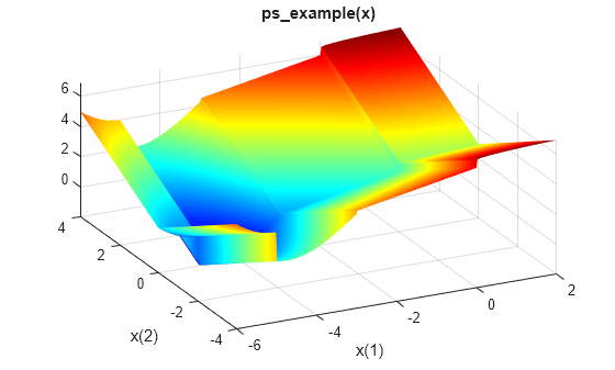
この例を実行すると、ps_example.m ファイルが含まれます。関数をプロットします。

xi = linspace(-6,2,300);
yi = linspace(-4,4,300);
[X,Y] = meshgrid(xi,yi);
Z = ps_example([X(:),Y(:)]);
Z = reshape(Z,size(X));
surf(X,Y,Z,'MeshStyle','none')
colormap 'jet'
view(-26,43)
xlabel('x(1)')
ylabel('x(2)')
title('ps\_example(x)')

ga を使用してこの関数の最小値を見つけます。

rng default % For reproducibility
x = ga(@ps_example,2)

ga stopped because the average change in the fitness value is less than options.FunctionTolerance.

x = 1×2

   -4.6793   -0.0860

線形制約付きの非滑らかな関数の最小化

遺伝的アルゴリズムを使用して、領域 x(1) + x(2) >= 1 および x(2) <= 5 + x(1) 上の ps_example 関数を最小化します。この関数は、この例を実行するときに含められます。

まず、2 つの不等式制約を行列形式 A*x <= b に変換します。つまり、不等式の左側の x 変数を取得し、両方の不等式が以下になるようにします。

-x(1) -x(2) <= -1

-x(1) + x(2) <= 5

A = [-1,-1;
    -1,1];
b = [-1;5];

ga を使用して制約問題を解きます。

rng default % For reproducibility
fun = @ps_example;
x = ga(fun,2,A,b)

ga stopped because the average change in the fitness value is less than options.FunctionTolerance.

x = 1×2

    0.9990    0.0000

制約は、制約許容値のデフォルト値 1e-3 内で満たされます。これを確認するには、負の要素を持つ A*x' - b を計算します。

disp(A*x' - b)

    0.0010
   -5.9990

線形等式および不等式制約を持つ非滑らかな関数の最小化

遺伝的アルゴリズムを使用して、領域 x(1) + x(2) >= 1 および x(2) == 5 + x(1) 上の ps_example 関数を最小化します。この関数は、この例を実行するときに含められます。

まず、2 つの制約を行列形式 A*x <= b と Aeq*x = beq に変換します。つまり、式の左側にある x 変数を取得し、不等式を以下という形式にします。

-x(1) -x(2) <= -1

-x(1) + x(2) == 5

A = [-1 -1];
b = -1;
Aeq = [-1 1];
beq = 5;

ga を使用して制約問題を解きます。

rng default % For reproducibility
fun = @ps_example;
x = ga(fun,2,A,b,Aeq,beq)

ga stopped because the average change in the fitness value is less than options.FunctionTolerance.

x = 1×2

   -2.0005    2.9995

制約がデフォルト値 ConstraintTolerance、1e-3 内で満たされていることを確認します。

disp(A*x' - b)

   1.0000e-03

disp(Aeq*x' - beq)

   8.5897e-09

線形制約と境界による最適化

遺伝的アルゴリズムを使用して、領域 x(1) + x(2) >= 1 および x(2) == 5 + x(1) 上の ps_example 関数を最小化します。この例を実行すると、ps_example 関数が含まれます。さらに、境界 1 <= x(1) <= 6 と -3 <= x(2) <= 8 を設定します。

まず、2 つの線形制約を行列形式 A*x <= b と Aeq*x = beq に変換します。つまり、式の左側にある x 変数を取得し、不等式を以下という形式にします。

-x(1) -x(2) <= -1

-x(1) + x(2) == 5

A = [-1 -1];
b = -1;
Aeq = [-1 1];
beq = 5;

境界 lb と ub を設定します。

lb = [1 -3];
ub = [6 8];

ga を使用して制約問題を解きます。

rng default % For reproducibility
fun = @ps_example;
x = ga(fun,2,A,b,Aeq,beq,lb,ub)

ga stopped because the average change in the fitness value is less than options.FunctionTolerance.

x = 1×2

    1.0000    6.0000

線形制約がデフォルト値 ConstraintTolerance、1e-3 内で満たされていることを確認します。

disp(A*x' - b)

   -6.0000

disp(Aeq*x' - beq)

  -7.9765e-08

ga を使用した非線形制約による最適化

遺伝的アルゴリズムを使用して、領域 $2{\mathit{x}}_1^2+{\mathit{x}}_2^2\le 3$ および $$(x_1+1{)}^2=(x_2/2{)}^4$$ 上の ps_example 関数を最小化します。この例を実行すると、ps_example 関数が含まれます。

これを行うには、最初の出力 c に不等式制約を返し、2 番目の出力 ceq に等式制約を返す関数 ellipsecons.m を使用します。この例を実行すると、ellipsecons 関数が含まれます。ellipsecons コードを調べます。

type ellipsecons

function [c,ceq] = ellipsecons(x)

c = 2*x(1)^2 + x(2)^2 - 3;
ceq = (x(1)+1)^2 - (x(2)/2)^4;

nonlcon 引数として ellipsecons への関数ハンドルを含めます。

nonlcon = @ellipsecons;
fun = @ps_example;
rng default % For reproducibility
x = ga(fun,2,[],[],[],[],[],[],nonlcon)

Optimization finished: average change in the fitness value less than options.FunctionTolerance and constraint violation is less than options.ConstraintTolerance.

x = 1×2

   -0.9766    0.0362

x で非線形制約が満たされていることを確認します。制約は、c ≤ 0 かつ ceq = 0 で、ConstraintTolerance、1e-3 のデフォルト値の範囲内である場合に満たされます。

[c,ceq] = nonlcon(x)

c = 
-1.0911

ceq = 
5.4645e-04

デフォルト以外のオプションで最小化

遺伝的アルゴリズムを使用して、デフォルトよりも小さい制約許容値を使用して、領域 x(1) + x(2) >= 1 および x(2) == 5 + x(1) 上の ps_example 関数を最小化します。この例を実行すると、ps_example 関数が含まれます。

まず、2 つの制約を行列形式 A*x <= b と Aeq*x = beq に変換します。つまり、式の左側にある x 変数を取得し、不等式を以下という形式にします。

-x(1) -x(2) <= -1

-x(1) + x(2) == 5

A = [-1 -1];
b = -1;
Aeq = [-1 1];
beq = 5;

より正確なソリューションを得るには、制約許容値を 1e-6 に設定します。ソルバーの進行状況を監視するには、プロット関数を設定します。

options = optimoptions('ga','ConstraintTolerance',1e-6,'PlotFcn', @gaplotbestf);

最小化問題を解きます。

rng default % For reproducibility
fun = @ps_example;
x = ga(fun,2,A,b,Aeq,beq,[],[],[],options)

ga stopped because the average change in the fitness value is less than options.FunctionTolerance.

x = 1×2

   -2.0000    3.0000

線形制約が 1e-6 以内で満たされていることを確認します。

disp(A*x' - b)

   9.9809e-07

disp(Aeq*x' - beq)

  -7.3589e-08

整数制約付きの非線形関数の最小化

遺伝的アルゴリズムを使用して、x(1) が整数であるという制約に従って ps_example 関数を最小化します。この関数は、この例を実行するときに含められます。

intcon = 1;
rng default % For reproducibility
fun = @ps_example;
A = [];
b = [];
Aeq = [];
beq = [];
lb = [];
ub = [];
nonlcon = [];
x = ga(fun,2,A,b,Aeq,beq,lb,ub,nonlcon,intcon)

ga stopped because the average change in the penalty function value is less than options.FunctionTolerance and 
the constraint violation is less than options.ConstraintTolerance.

x = 1×2

   -5.0000   -0.0834

解と関数値を取得する

遺伝的アルゴリズムを使用して、整数制約の非線形問題を最小化します。最小値の位置と最小関数値の両方を取得します。この例を実行すると、目的関数 ps_example が含まれます。

intcon = 1;
rng default % For reproducibility
fun = @ps_example;
A = [];
b = [];
Aeq = [];
beq = [];
lb = [];
ub = [];
nonlcon = [];
[x,fval] = ga(fun,2,A,b,Aeq,beq,lb,ub,nonlcon,intcon)

ga stopped because the average change in the penalty function value is less than options.FunctionTolerance and 
the constraint violation is less than options.ConstraintTolerance.

x = 1×2

   -5.0000   -0.0834

fval = 
-1.8344

この結果を、制約のない問題の解決と比較します。

[x,fval] = ga(fun,2)

ga stopped because the average change in the fitness value is less than options.FunctionTolerance.

x = 1×2

   -4.6906   -0.0078

fval = 
-1.9918

診断情報を取得する

遺伝的アルゴリズムを使用して、x(1) が整数値になるように制約された ps_example 関数を最小化します。この例を実行すると、ps_example 関数が含まれます。ソルバーが停止した理由と ga が最小値をどのように探索したかを理解するには、exitflag と output の結果を取得します。また、ソルバーが進行するにつれて、観測された目的関数の最小値をプロットします。

intcon = 1;
rng default % For reproducibility
fun = @ps_example;
A = [];
b = [];
Aeq = [];
beq = [];
lb = [];
ub = [];
nonlcon = [];
options = optimoptions('ga','PlotFcn', @gaplotbestf);
[x,fval,exitflag,output] = ga(fun,2,A,b,Aeq,beq,lb,ub,nonlcon,intcon,options)

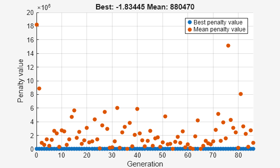
ga stopped because the average change in the penalty function value is less than options.FunctionTolerance and 
the constraint violation is less than options.ConstraintTolerance.

x = 1×2

   -5.0000   -0.0834

fval = 
-1.8344

exitflag = 
1

output = struct with fields:
      problemtype: 'integerconstraints'
         rngstate: [1×1 struct]
      generations: 86
        funccount: 3311
          message: 'ga stopped because the average change in the penalty function value is less than options.FunctionTolerance and ↵the constraint violation is less than options.ConstraintTolerance.'
    maxconstraint: 0
       hybridflag: []

最終的な母集団とスコアを取得する

遺伝的アルゴリズムを使用して、x(1) が整数値になるように制約された ps_example 関数を最小化します。この例を実行すると、ps_example 関数が含まれます。最終的な母集団とスコアのベクトルを含むすべての出力を取得します。

intcon = 1;
rng default % For reproducibility
fun = @ps_example;
A = [];
b = [];
Aeq = [];
beq = [];
lb = [];
ub = [];
nonlcon = [];
[x,fval,exitflag,output,population,scores] = ga(fun,2,A,b,Aeq,beq,lb,ub,nonlcon,intcon);

ga stopped because the average change in the penalty function value is less than options.FunctionTolerance and 
the constraint violation is less than options.ConstraintTolerance.

最終的な母集団の最初の 10 人のメンバーとそれに対応するスコアを調べます。これらすべての母集団メンバーについて、x(1) は整数値であることに注意してください。整数 ga アルゴリズムは整数実行可能な母集団のみを生成します。

disp(population(1:10,:))

   1.0e+03 *

   -0.0050   -0.0001
   -0.0050   -0.0001
   -1.6420    0.0027
   -1.5070    0.0010
   -0.4540    0.0104
   -0.2530   -0.0011
   -0.1210   -0.0003
   -0.1040    0.1314
   -0.0140   -0.0010
    0.0160   -0.0002

disp(scores(1:10))

   1.0e+06 *

   -0.0000
   -0.0000
    2.6798
    2.2560
    0.2016
    0.0615
    0.0135
    0.0099
    0.0001
    0.0000

入力引数

fun — 目的関数

関数ハンドル | 関数名

関数ハンドルまたは関数名として指定される目的関数。長さ nvars の行ベクトルを受け入れ、スカラー値を返す目的関数を記述します。

'UseVectorized' オプションが true の場合、pop 行 nvars 列の行列を受け入れるには fun と記述します。ここで、pop は現在の母集団サイズです。この場合、fun は、適応度関数の値を含む pop と同じ長さのベクトルを返します。ga はベクトル化された計算でも母集団の単一のメンバーを渡すことができるため、fun が pop に対して特定のサイズを想定していないことを確認してください。

例: fun = @(x)(x-[4,2]).^2

データ型: char | function_handle | string

nvars — 変数の数

正の整数

変数の数。正の整数として指定されます。ソルバーは長さが nvars から fun までの行ベクトルを渡します。

例: 4

データ型: double

A — 線形不等式制約

実数行列

線形不等式制約。実数行列として指定されます。A は M 行 nvars 列の行列で、M は不等式の数です。

A は M 個の線形不等式を符号化します。

A*x <= b,

ここで、x は nvars 個の変数 x(:) の列ベクトル、b は M 個の要素をもつ列ベクトルです。

例えば、

x₁ + 2x₂ ≤ 10
3x₁ + 4x₂ ≤ 20
5x₁ + 6x₂ ≤ 30,

次の制約を与えます:

A = [1,2;3,4;5,6];
b = [10;20;30];

例: 制御変数の合計が 1 以下になるように指定するには、制約 A = ones(1,N) と b = 1 を指定します。

データ型: double

b — 線形不等式制約

実数ベクトル

実数ベクトルで指定される線形不等式制約です。b は、行列 A に関連する M 要素ベクトルです。b を行ベクトルとして渡す場合、ソルバーは b を列ベクトル b(:) に内部的に変換します。

b は M 個の線形不等式を符号化します。

A*x <= b,

ここで、x は N 個の変数 x(:) の列ベクトル、A は M 行 N 列の行列です。

例えば、

x₁ + 2x₂ ≤ 10
3x₁ + 4x₂ ≤ 20
5x₁ + 6x₂ ≤ 30,

次の制約を与えます:

A = [1,2;3,4;5,6];
b = [10;20;30];

例: 制御変数の合計が 1 以下になるように指定するには、制約 A = ones(1,N) と b = 1 を指定します。

データ型: double

Aeq — 線形等式制約

実数行列

線形等式制約。実数行列として指定されます。Aeq は Me 行 nvars 列の行列で、Me は等式の数です。

Aeq は Me 個の線形等式を符号化します。

Aeq*x = beq,

ここで、x は N 個の変数 x(:) の列ベクトル、beq は Me 個の要素をもつ列ベクトルです。

例えば、

x₁ + 2 x₂ + 3 x₃ = 10
2 x₁ + 4 x₂ + x₃ = 20,

次の制約を与えます:

Aeq = [1,2,3;2,4,1];
beq = [10;20];

例: 制御変数の合計が 1 になるように指定するには、制約 Aeq = ones(1,N) と beq = 1 を指定します。

データ型: double

beq — 線形等式制約

実数ベクトル

実数ベクトルで指定される線形等式制約です。beq は、行列 Aeq に関連する Me 要素ベクトルです。beq を行ベクトルとして渡す場合、ソルバーは beq を列ベクトル beq(:) に内部的に変換します。

beq は Me 個の線形等式を符号化します。

Aeq*x = beq,

ここで、x は N 個の変数 x(:) の列ベクトル、Aeq は Meq 行 N 列の行列です。

例えば、

x₁ + 2 x₂ + 3 x₃ = 10
2 x₁ + 4 x₂ + x₃ = 20,

次の制約を与えます:

Aeq = [1,2,3;2,4,1];
beq = [10;20];

例: 制御変数の合計が 1 になるように指定するには、制約 Aeq = ones(1,N) と beq = 1 を指定します。

データ型: double

lb — 下限

[] (既定値) | 実数ベクトルまたは配列

下限は、実数ベクトルまたは double の配列として指定されます。lb は、lb ≤ x ≤ ub 内の要素ごとの下限を表します。

ga は配列 lb をベクトル lb(:) に内部的に変換します。

例: lb = [0;-Inf;4] は x(1) ≥ 0, x(3) ≥ 4 を意味します。

データ型: double

ub — 上限

[] (既定値) | 実数ベクトルまたは配列

上限は、実数ベクトルまたは double の配列として指定されます。ub は、lb ≤ x ≤ ub 内の要素ごとの上限を表します。

ga は配列 ub をベクトル ub(:) に内部的に変換します。

例: ub = [Inf;4;10] は x(2) ≤ 4, x(3) ≤ 10 を意味します。

データ型: double

nonlcon — 非線形制約

関数ハンドル | 関数名

非線形制約。関数ハンドルまたは関数名として指定されます。nonlcon は、ベクトルまたは配列 x を受け、2 つの配列 c(x) および ceq(x) を返す関数です。

• c(x) は、x での非線形不等式制約の配列です。ga は次の条件を満たそうとします。

  c(x) <= 0

  c のすべてのエントリについて。

• ceq(x) は、x での非線形等式制約の配列です。ga は次の条件を満たそうとします。

  ceq(x) = 0

  ceq のすべてのエントリについて。

以下に例を示します。

x = ga(@myfun,4,A,b,Aeq,beq,lb,ub,@mycon)

ここで mycon は次のような MATLAB^® 関数です。

function [c,ceq] = mycon(x)
c = ...     % Compute nonlinear inequalities at x.
ceq = ...   % Compute nonlinear equalities at x.

詳細については、非線形制約を参照してください。

ベクトル化された制約の使用方法については、ベクトル化された制約 を参照してください。

メモ

ga は、PopulationType オプションが 'bitString' または 'custom' に設定されている場合に、非線形制約を満たすことを強制しません。

intcon が空でない場合、nonlcon の 2 番目の出力 (ceq) は空のエントリ ([]) である必要があります。

ga が nonlcon を使用する方法については、遺伝的アルゴリズムのための非線形制約ソルバーアルゴリズム を参照してください。

データ型: char | function_handle | string

options — 最適化オプション

optimoptions の出力 | 構造体

最適化オプション。optimoptions の出力または構造体として指定されます。

optimoptions は、斜体 でリストされているオプションを非表示にします。optimoptions で非表示になっているオプションを参照してください。

• {} 内の値はデフォルト値を示します。

• {}* は線形制約がある場合のデフォルトを表し、MutationFcn は境界がある場合のデフォルトを表します。

• I* は、整数制約のデフォルトを示すか、整数制約に関する特別な考慮事項を示します。

• NM は、オプションが gamultiobj には適用されないことを示します。

ga と gamultiobj のオプション

オプション	説明	値
ConstraintTolerance	非線形制約に関する実現可能性を決定します。また、max(sqrt(eps),ConstraintTolerance) は線形制約に関して実現可能性を決定します。 オプション構造の場合は、TolCon を使用します。	非負のスカラー | {1e-3}
CreationFcn	初期母集団を作成する関数。組み込み作成関数または関数ハンドルの名前として指定します。母集団オプションを参照してください。	{'gacreationuniform'} | {'gacreationlinearfeasible'}* | 'gacreationnonlinearfeasible' | {'gacreationuniformint'}I* for ga | {'gacreationsobol'}I* for gamultiobj | カスタム作成機能
CrossoverFcn	アルゴリズムが交叉子を作成するために使用する関数。組み込み交叉関数または関数ハンドルの名前として指定します。交叉オプションを参照してください。	{'crossoverscattered'} は ga、{'crossoverintermediate'}* は gamultiobj です | {'crossoverlaplace'}I* | 'crossoverheuristic' | 'crossoversinglepoint' | 'crossovertwopoint' | 'crossoverarithmetic' | カスタム交叉機能
CrossoverFraction	交叉関数によって生成される、エリートの子供を含まない世代の母集団の割合。	非負のスカラー | {0.8}
Display	表示レベル。	'off' | 'iter' | 'diagnose' | {'final'}
DistanceMeasureFcn	個体の距離を計算する関数。組み込みの距離測定関数または関数ハンドルの名前として指定します。値は、決定変数または設計空間 (遺伝子型) または機能空間 (表現型) に適用されます。デフォルトの 'distancecrowding' は関数空間 (表現型) にあります。gamultiobj のみ。多目的オプションを参照してください。 オプション構造体の場合は、名前ではなく関数ハンドルを使用します。	{'distancecrowding'} は {@distancecrowding,'phenotype'} と同じ意味です | {@distancecrowding,'genotype'} | カスタム距離関数
EliteCount	NM 現在の世代の個体のうち、次の世代まで生き残ることが保証されている個体の数を指定する正の整数。gamultiobjでは使用されません。	非負整数 | {ceil(0.05*PopulationSize)} | 混合整数問題の場合は {0.05*(default PopulationSize)}
FitnessLimit	NM適応度関数が FitnessLimit の値に達すると、アルゴリズムは停止します。	スカラー | {-Inf}
FitnessScalingFcn	適応度関数の値をスケーリングする関数。組み込みスケーリング関数または関数ハンドルの名前として指定します。gamultiobj ではオプションは使用できません。	{'fitscalingrank'} | 'fitscalingshiftlinear' | 'fitscalingprop' | 'fitscalingtop' | カスタムフィットネススケーリング関数
FunctionTolerance	MaxStallGenerations世代にわたる最良の適応度関数値の平均相対変化が FunctionTolerance 以下になった場合、アルゴリズムは停止します。StallTest が 'geometricWeighted' の場合、加重平均相対変化が FunctionTolerance 以下であればアルゴリズムは停止します。 gamultiobj の場合、options.MaxStallGenerations世代にわたる広がり値の相対的変化の幾何平均が options.FunctionTolerance より小さくなり、最終的な広がりが過去の options.MaxStallGenerations世代にわたる平均広がりより小さくなったときにアルゴリズムは停止します。gamultiobj アルゴリズムを参照してください。 オプション構造の場合は、TolFun を使用します。	非負のスカラー | ga の場合は {1e-6}、gamultiobj の場合は {1e-4}
HybridFcn	I* ga が終了した後も最適化を継続する関数。名前または関数ハンドルとして指定します。 または、ハイブリッド関数とそのオプションを指定するセル配列。gaハイブリッド関数を参照してください。 gamultiobj の場合、唯一のハイブリッド関数は @fgoalattain です。gamultiobjハイブリッド関数を参照してください。 問題に整数制約がある場合は、ハイブリッド関数は使用できません。 ハイブリッド関数を使用する場合を参照してください。	関数名またはハンドル | 'fminsearch' | 'patternsearch' | 'fminunc' | 'fmincon' | {[]} または 1行2列のセル配列 | {@solver, hybridoptions}（solver = fminsearch、patternsearch、fminunc、またはfmincon {[]}）
InitialPenalty	NM I* ペナルティパラメーターの初期値	正のスカラー | {10}
InitialPopulationMatrix	遺伝的アルゴリズムのシードに使用される初期母集団。最大 PopulationSize 行、N 列です。ここで、N は変数の数です。部分的な母集団、つまり PopulationSize 行未満の母集団を渡すことができます。その場合、遺伝的アルゴリズムは CreationFcn を使用して残りの母集団メンバーを生成します。母集団オプションを参照してください。 オプション構造の場合は、InitialPopulation を使用します。	行列 | {[]}
InitialPopulationRange	初期母集団内の個体の範囲を指定する行列またはベクトル。gacreationuniform 作成関数に適用されます。ga は、デフォルトの初期範囲をシフトおよびスケーリングして、有限の境界に一致させます。 オプション構造の場合は、PopInitRange を使用します。	行列またはベクトル | {[-10;10]} は非有界成分、{[-1e4+1;1e4+1]} は整数制約問題の非有界成分、{[lb;ub]} は有界成分、デフォルトの範囲は片側境界に合わせて変更されます
InitialScoresMatrix	適応度を決定するために使用される初期スコア。最大 PopulationSize 行、Nf 列があります。ここで、Nf は適応度関数の数です (ga の場合は 1、gamultiobj の場合は 1 より大きくなります)。部分スコア行列 (つまり、PopulationSize 行未満の行列) を渡すことができます。その場合、ソルバーは適応度関数を評価するときにスコアを入力します。 オプション構造の場合は、InitialScores を使用します。	単一目的の列ベクトル | 多目的の行列 | {[]}
MaxGenerations	アルゴリズムが停止するまでの最大反復回数。 オプション構造の場合は、Generations を使用します。	非負整数 |{100*numberOfVariables} は ga、{200*numberOfVariables} は gamultiobj
MaxStallGenerations	MaxStallGenerations世代にわたる最良の適応度関数値の平均相対変化が FunctionTolerance 以下になった場合、アルゴリズムは停止します。StallTest が 'geometricWeighted' の場合、加重平均相対変化が FunctionTolerance 以下であればアルゴリズムは停止します。 gamultiobj の場合、options.MaxStallGenerations世代にわたる広がり値の相対的変化の幾何平均が options.FunctionTolerance より小さくなり、最終的な広がりが過去の options.MaxStallGenerations世代にわたる平均広がりより小さくなったときにアルゴリズムは停止します。gamultiobj アルゴリズムを参照してください。 オプション構造の場合は、StallGenLimit を使用します。	非負の整数 | ga の場合は {50}、gamultiobj の場合は {100}
MaxStallTime	NM tic と toc で測定された MaxStallTime 秒間に目的関数の改善が見られない場合、アルゴリズムは停止します。 オプション構造の場合は、StallTimeLimit を使用します。	正のスカラー | {Inf}
MaxTime	アルゴリズムは、tic と toc で測定された MaxTime 秒間実行された後に停止します。この制限は各反復の後に適用されるため、反復にかなりの時間がかかる場合は ga が制限を超える可能性があります。 オプション構造の場合は、TimeLimit を使用します。	非負のスカラー | {Inf}
MigrationDirection	移行の方向。移行オプションを参照してください。	'both' | {'forward'}
MigrationFraction	各サブ集団内で別のサブ集団に移動する個体の割合を指定する 0 から 1 までのスカラー。移行オプションを参照してください。	スカラー | {0.2}
MigrationInterval	個体がサブポピュレーション間で移動する間に発生する世代数を指定する正の整数。移行オプションを参照してください。	正の整数 | {20}
MutationFcn	突然変異の子を生成する関数。組み込みの突然変異関数または関数ハンドルの名前として指定します。突然変異オプションを参照してください。	制約なしの ga の {'mutationgaussian'} | 制約ありの gamultiobj および ga の {'mutationadaptfeasible'}* | {'mutationpower'}I* | 'mutationpositivebasis' | 'mutationuniform' | カスタム突然変異関数
NonlinearConstraintAlgorithm	非線形制約アルゴリズム。遺伝的アルゴリズムのための非線形制約ソルバーアルゴリズムを参照してください。gamultiobj ではオプションは変更できません。 オプション構造の場合は、NonlinConAlgorithm を使用します。	ga では {'auglag'}、gamultiobj では {'penalty'}
OutputFcn	ga が各反復で呼び出す関数。関数ハンドルまたは関数ハンドルのセル配列として指定します。出力関数のオプションを参照してください。 オプション構造の場合は、OutputFcns を使用します。	関数ハンドルまたは関数ハンドルのセル配列 | {[]}
ParetoFraction	gamultiobj の場合のみ、ソルバーがより高いフロントから個体を選択している間、最初のパレート フロントに保持する個体の割合を指定する 0 から 1 までのスカラー。多目的オプションを参照してください。	スカラー | {0.35}
PenaltyFactor	NM I* ペナルティ更新パラメーター。	正のスカラー | {100}
PlotFcn	アルゴリズムによって計算されたデータをプロットする関数。組み込みプロット関数の名前、関数ハンドル、または組み込みの名前や関数ハンドルのセル配列として指定します。プロット オプションを参照してください。 オプション構造の場合は、PlotFcns を使用します。	ga または gamultiobj:{[]} | 'gaplotdistance' | 'gaplotgenealogy' | 'gaplotselection' | 'gaplotscorediversity' |'gaplotscores' | 'gaplotstopping' | 'gaplotmaxconstr' | カスタム プロット関数 gaのみ: 'gaplotbestf' | 'gaplotbestindiv' | 'gaplotexpectation' | 'gaplotrange' gamultiobjのみ: 'gaplotpareto' | 'gaplotparetodistance' | 'gaplotrankhist' | 'gaplotspread'
PlotInterval	プロット関数の連続呼び出し間の世代数を指定する正の整数。	正の整数 | {1}
PopulationSize	母集団の規模。	正の整数 | numberOfVariables <= 5の場合は{50}、それ以外の場合は{200} | 混合整数問題の場合のみga、{min(max(10*nvars,40),100)}
PopulationType	母集団のデータ型。混合整数問題の場合は 'doubleVector' にする必要があります。	'bitstring' | 'custom' | {'doubleVector'} PopulationType が 'bitString' または 'custom' に設定されている場合、ga はすべての制約を無視します。母集団オプションを参照してください。
SelectionFcn	交叉および突然変異の子の親を選択する関数。組み込み選択関数または関数ハンドルの名前として指定します。 gamultiobj は 'selectiontournament' またはカスタム選択機能のみを使用します。	{'selectionstochunif'} は ga、{'selectiontournament'} は gamultiobj です | 'selectionremainder' | 'selectionuniform' | 'selectionroulette' | カスタム選択機能
StallTest	NMテストタイプを停止しています。	'geometricWeighted' | {'averageChange'}
UseParallel	適応度と非線形制約関数を並列に計算します。ベクトル化と並列化オプション（ユーザー関数評価）とGlobal Optimization Toolbox で並列処理を使用する方法を参照してください。	true | {false}
UseVectorized	関数がベクトル化されるかどうかを指定します。ベクトル化と並列化オプション（ユーザー関数評価）と適応度関数をベクトル化するを参照してください。 オプション構造の場合は、値 'on' または 'off' とともに Vectorized を使用します。	true | {false}

例: optimoptions('ga','PlotFcn',@gaplotbestf)

intcon — 整数変数

正の整数のベクトル

整数変数。1 から nvars までの値を取る正の整数のベクトルとして指定されます。intcon の各値は、整数値の x コンポーネントを表します。

メモ

intcon が空でない場合、nonlcon は ceq に対して空を返す必要があります。整数計画法の詳細については、混合整数ga最適化 を参照してください。

例: xの偶数エントリが整数値であることを指定するには、intconを2:2:nvarsに設定します。

データ型: double

problem — 問題の説明

構造体

問題の説明。これらのフィールドを含む構造体として指定されます。

fitnessfcn	適応度関数
nvars	設計変数の数
Aineq	線形不等式制約のA行列
Bineq	線形不等式制約のbベクトル
Aeq	線形等式制約のAeq行列
Beq	線形等式制約のbeqベクトル
lb	xの下限
ub	xの上限
nonlcon	非線形制約関数
intcon	整数変数のインデックス
rngstate	乱数ジェネレータの状態をリセットするフィールド
solver	'ga'
options	optimoptions またはオプション構造を使用して作成されたオプション

フィールド fitnessfcn、nvars、および options を指定する必要があります。残りは ga ではオプションです。

データ型: struct

出力引数

x — 解

実数ベクトル

解は実数ベクトルとして返されます。x は、ga が反復中に特定した最適なポイントです。

fval — 解での目的関数値

実数

解での目的関数値。実数として返されます。一般的に、fval = fun(x) になります。

exitflag — ga の停止理由

整数

ga が停止した理由が整数として返されます。

終了フラグ	意味
1	"非線形制約なし" — MaxStallGenerations 世代にわたる適応度関数の値の平均累積変化が FunctionTolerance より小さく、制約違反が ConstraintTolerance より小さいことを示します。
	"非線形制約あり" — 相補性測度 (相補性測度を参照) の大きさが sqrt(ConstraintTolerance) より小さく、部分問題を解くのに FunctionTolerance より小さい許容誤差が使用され、制約違反が ConstraintTolerance より小さいことを示します。
3	適応度関数の値が MaxStallGenerations 世代内で変化せず、制約違反が ConstraintTolerance より小さいことを示します。
4	ステップの大きさはマシン精度より小さく、制約違反は ConstraintTolerance 未満です。
5	適応度の下限 FitnessLimit に到達しており、制約違反が ConstraintTolerance より小さいことを示します。
0	世代 MaxGenerations の最大数を超過していることを示します。
-1	出力関数またはプロット関数によって最適化が停止したことを示します。
-2	実行可能点が検出されませんでした。
-4	停滞時間制限 MaxStallTime を超えていることを示します。
-5	制限時間 MaxTime を超えていることを示します。

整数制約がある場合、ga は停止基準として適応度値ではなくペナルティ適合度値を使用します。

output — 最適化プロセスに関する情報

構造体

最適化プロセスに関する情報。次のフィールドをもつ構造体として返されます。

• problemtype — 問題の種類。次のいずれかです:

  • 'unconstrained'

  • 'boundconstraints'

  • 'linearconstraints'

  • 'nonlinearconstr'

  • 'integerconstraints'

• rngstate — アルゴリズムが開始する直前の MATLAB 乱数ジェネレーターの状態。rngstate の値を使用して、ga の出力を再現できます。結果を再現するを参照してください。

• generations — 計算された世代数。

• funccount —適応度関数の評価回数。

• message — アルゴリズムが終了した理由。

• maxconstraint — 最大制約違反（ある場合）。

• hybridflag —ハイブリッド関数からの終了フラグ。HybridFcn options に関連します。gamultiobjには適用されません。

population — 最終母集団

行列

最終的な母集団は、PopulationSize 行 nvars 列の行列として返されます。population の行は個体です。

scores — 最終スコア

列ベクトル

最終スコアは列ベクトルとして返されます。

• 非整数問題の場合、最終スコアは population の行の適応度関数値になります。

• 整数問題の場合、最終スコアは母集団メンバーのペナルティ適応度値になります。整数gaアルゴリズムを参照してください。

詳細

相補性測度

拡張ラグランジュ非線形制約ソルバーでは、相補性尺度は、要素が c_iλ_i であるベクトルのノルムです。ここで、c_i は非線形不等式制約違反であり、λ_i は対応するラグランジュ乗数です。拡張ラグランジュ遺伝的アルゴリズムを参照してください。

ヒント

• ga によって呼び出すことができる独立変数への追加パラメーターを持つ関数を記述するには、追加パラメーターの受け渡し を参照してください。

• 母集団タイプ Double Vector (デフォルト) を使用する問題の場合、ga は入力がタイプ complex である関数を受け入れません。複雑なデータを含む問題を解決するには、実数部と虚数部を分離して、実数ベクトルを受け入れるように関数を記述します。

アルゴリズム

遺伝的アルゴリズムの説明については、遺伝的アルゴリズムの仕組み を参照してください。

混合整数計画アルゴリズムの説明については、整数gaアルゴリズム を参照してください。

非線形制約アルゴリズムの説明については、遺伝的アルゴリズムのための非線形制約ソルバーアルゴリズム を参照してください。

代替機能

アプリ

最適化ライブ エディター タスクが ga にビジュアル インターフェイスを提供します。

参照

[1] Goldberg, David E., Genetic Algorithms in Search, Optimization & Machine Learning, Addison-Wesley, 1989.

[2] A. R. Conn, N. I. M. Gould, and Ph. L. Toint. “A Globally Convergent Augmented Lagrangian Algorithm for Optimization with General Constraints and Simple Bounds”, SIAM Journal on Numerical Analysis, Volume 28, Number 2, pages 545–572, 1991.

[3] A. R. Conn, N. I. M. Gould, and Ph. L. Toint. “A Globally Convergent Augmented Lagrangian Barrier Algorithm for Optimization with General Inequality Constraints and Simple Bounds”, Mathematics of Computation, Volume 66, Number 217, pages 261–288, 1997.

拡張機能

自動並列サポート

Parallel Computing Toolbox™ を使用して自動的に並列計算を実行することで、コードを高速化します。

並列実行するには、'UseParallel' オプションを true に設定します。

options = optimoptions('solvername','UseParallel',true)

詳細については、Global Optimization Toolbox で並列処理を使用する方法を参照してください。

バージョン履歴

R2006a より前に導入

R2019b: ga は適応度関数評価回数が少なくなります

適応度関数が決定論的である場合、ga はエリート (現在最良の)個体に対して適応度関数を再評価しません。この動作を制御するには、新しい state.EvalElites フィールドにアクセスし、カスタム出力関数またはカスタム プロット関数で変更します。同様に、初期母集団に重複するメンバーがある場合、ga は各一意のメンバーを 1 回だけ評価します。新しい state.HaveDuplicates フィールドにアクセスして変更することにより、カスタム出力関数またはカスタム プロット関数でこの動作を制御できます。詳細については、遺伝的アルゴリズムのカスタム出力関数 または カスタム プロット関数 を参照してください。

2 つの新しいフィールドの詳細については、状態構造 を参照してください。

参考

gamultiobj | optimoptions | particleswarm | patternsearch | 最適化

トピック

• 遺伝的アルゴリズム
• Global Optimization Toolbox を使い始める
• ソルバーベースの最適化問題の設定