YOLO v3 深層学習を使用したオブジェクトの検出
この例では、You Only Look Once version 3 (YOLO v3) 深層学習ネットワークを使用して、イメージ内のオブジェクトを検出する方法を説明します。この例では、次の作業を行います。
YOLO v3 オブジェクト検出ネットワークの学習用とテスト用のデータセットを構成。また、ネットワーク効率を向上させるため、学習データセットのデータ拡張を実行。
yolov3ObjectDetector(Computer Vision Toolbox)関数を使用して YOLO v3 オブジェクト検出器を作成し、trainYOLOv3ObjectDetector(Computer Vision Toolbox)関数を使用して検出器の学習を実行。
この例では、イメージに含まれる車両を検出するための事前学習済みの YOLO v3 オブジェクト検出器についても説明します。この事前学習済みのネットワークは、バックボーン ネットワークとして SqueezeNet を使用し、車両データセットで学習を行っています。YOLO v3 オブジェクト検出ネットワークの詳細については、YOLO v3 入門 (Computer Vision Toolbox)を参照してください。
データの読み込み
この例では、295 個のイメージを含んだ小さなラベル付きデータセットを使用します。これらのイメージの多くは、Caltech の Cars 1999 データ セットおよび Cars 2001 データ セットからのものです。Pietro Perona 氏によって作成されたもので、許可を得て使用しています。各イメージには、1 または 2 個のラベル付けされた車両インスタンスが含まれています。小さなデータセットは YOLO v3 の学習手順を調べるうえで役立ちますが、実際にロバストなネットワークに学習させるにはラベル付けされたイメージがより多く必要になります。
車両のイメージを解凍し、車両のグラウンド トゥルース データを読み込みます。
unzip vehicleDatasetImages.zip
data = load("vehicleDatasetGroundTruth.mat");
vehicleDataset = data.vehicleDataset;
車両データは 2 列の table に保存されています。1 列目にはイメージ ファイルのパスが含まれ、2 列目には境界ボックスが含まれています。
データ セットの最初の数行を表示します。
vehicleDataset(1:4,:)
ans=4×2 table
    'vehicleImages/image_00001.jpg'    [220,136,35,28]
    'vehicleImages/image_00002.jpg'    [175,126,61,45]
    'vehicleImages/image_00003.jpg'    [108,120,45,33]
    'vehicleImages/image_00004.jpg'    [124,112,38,36]
ローカルの車両データ フォルダーへの絶対パスを追加します。
vehicleDataset.imageFilename = fullfile(pwd,vehicleDataset.imageFilename);
データセットは学習、検証、テスト用のセットに分割します。データの 60% を学習用に、10% を検証用に、残りを学習済みの検出器のテスト用に選択します。
rng(0);
shuffledIndices = randperm(height(vehicleDataset));
idx = floor(0.6 * length(shuffledIndices) );

trainingIdx = 1:idx;
trainingDataTbl = vehicleDataset(shuffledIndices(trainingIdx),:);

validationIdx = idx+1 : idx + 1 + floor(0.1 * length(shuffledIndices) );
validationDataTbl = vehicleDataset(shuffledIndices(validationIdx),:);

testIdx = validationIdx(end)+1 : length(shuffledIndices);
testDataTbl = vehicleDataset(shuffledIndices(testIdx),:);
imageDatastoreオブジェクトおよびboxLabelDatastore (Computer Vision Toolbox)オブジェクトを使用して、学習および評価中にイメージとラベル データを読み込むデータストアを作成します。
imdsTrain = imageDatastore(trainingDataTbl{:,"imageFilename"});
bldsTrain = boxLabelDatastore(trainingDataTbl(:,"vehicle"));

imdsValidation = imageDatastore(validationDataTbl{:,"imageFilename"});
bldsValidation = boxLabelDatastore(validationDataTbl(:,"vehicle"));

imdsTest = imageDatastore(testDataTbl{:,"imageFilename"});
bldsTest = boxLabelDatastore(testDataTbl(:,"vehicle"));
イメージ データストアとボックス ラベル データストアを組み合わせます。
trainingData = combine(imdsTrain,bldsTrain);
validationData = combine(imdsValidation,bldsValidation);
testData = combine(imdsTest,bldsTest);
この例に添付されている validateInputData サポート関数を使用して、次などの無効な入力データを検出します。
無効な形式のイメージ、または NaN を含むイメージ
ゼロ/NaN/Inf を含むか、空である境界ボックス
欠損ラベル/非カテゴリカル ラベル
境界ボックスの値は、有限、正、整数で、NaN 以外でなければなりません。また、正の高さと幅をもつイメージ境界内に収まらなくてはなりません。無効な入力データは、破棄するか、適切な学習のために修正しなければなりません。
validateInputData(trainingData);
validateInputData(validationData);
validateInputData(testData);
データ拡張
データ拡張は、学習中に元のデータをランダムに変換してネットワークの精度を高めるために使用されます。データ拡張を使用すると、ラベル付き学習サンプルの数を実際に増やさずに、学習データをさらに多様化させることができます。
関数 transform を使用して、カスタムのデータ拡張を学習データに適用します。augmentData 補助関数によって、入力データに以下の拡張が適用されます。
HSV 空間でのカラー ジッターの付加
水平方向のランダムな反転
10% のランダムなスケーリング
augmentedTrainingData = transform(trainingData,@augmentData);
同じイメージを 4 回読み取り、拡張された学習データを表示します。
augmentedData = cell(4,1);
for k = 1:4
    data = read(augmentedTrainingData);
    augmentedData{k} = insertShape(data{1,1},"Rectangle",data{1,2});
    reset(augmentedTrainingData);
end
figure
montage(augmentedData,BorderSize=10)
reset(augmentedTrainingData);
YOLO v3 オブジェクト検出器の定義
この例の YOLO v3 検出器は、SqueezeNet がベースとなっています。この検出器は、SqueezeNet の特徴抽出ネットワークを使用し、最後に 2 つの検出ヘッドが追加されています。2 番目の検出ヘッドのサイズは、最初の検出ヘッドの 2 倍となっているため、小さなオブジェクトをより的確に検出できます。検出したいオブジェクトのサイズに基づいて、サイズが異なる検出ヘッドを任意の数だけ指定できます。YOLO v3 検出器は、学習データを使用して推定されたアンカー ボックスを使用します。これにより、データ セットの種類に対応した初期の事前確率が改善され、ボックスを正確に予測できるように検出器に学習させることができます。アンカー ボックスの詳細については、アンカー ボックスによるオブジェクトの検出 (Computer Vision Toolbox)を参照してください。
YOLO v3 検出器内に存在する YOLO v3 ネットワークを次の図に示します。
ディープ ネットワーク デザイナーを使用して、この図に示されているネットワークを作成することができます。

ネットワーク入力サイズを指定します。ネットワーク入力サイズを選択する際には、ネットワーク自体の実行に必要な最小サイズ、学習イメージのサイズ、および選択したサイズでデータを処理することによって発生する計算コストを考慮します。可能な場合、学習イメージのサイズに近く、ネットワークに必要な入力サイズより大きいネットワーク入力サイズを選択します。この例の実行にかかる計算コストを削減するため、ネットワーク入力サイズを [227 227 3] に指定します。
networkInputSize = [227 227 3];
この例で使用されている学習イメージは、227×227 より大きく、サイズがまちまちであるため、まず、transform 関数を使用して、アンカー ボックスを計算するための学習データを前処理します。アンカーの数と平均 Intersection over Union (IoU) との良好なトレードオフを実現するため、アンカーの数を 6 に指定します。estimateAnchorBoxes 関数を使用して、アンカー ボックスの数と平均 IoU 値を推定します。アンカー ボックスの推定の詳細については、学習データからのアンカー ボックスの推定 (Computer Vision Toolbox)を参照してください。事前学習済みの YOLOv3 オブジェクト検出器を使用する場合、特定の学習データセットで計算されたアンカー ボックスを指定する必要があります。推定プロセスは確定的なものではないことに注意してください。推定されたアンカー ボックスが他のハイパーパラメーターの調整中に変化しないように、rng 関数を使用して推定前に乱数シードを設定します。
rng(0)
trainingDataForEstimation = transform(trainingData,@(data)preprocessData(data,networkInputSize));
numAnchors = 6;
[anchors,meanIoU] = estimateAnchorBoxes(trainingDataForEstimation,numAnchors)
anchors = 6×2

     42     37
    160    130
     96     92
    141    123
     35     25
     69     66
meanIoU =
0.8430
両方の検出ヘッドで使用する anchorBoxes を指定します。anchorBoxes は、M 行 1 列の cell 配列です。ここで、M は検出ヘッドの数を表します。各検出ヘッドは、anchors の N 行 2 列の行列で構成されます。ここで、N は使用するアンカーの数です。特徴マップのサイズに基づいて、各検出ヘッドの anchorBoxes を選択します。スケールが小さい場合は大きい anchors を使用し、スケールが大きい場合は小さい anchors を使用します。これを行うには、より大きいアンカー ボックスが先頭に来るように anchors を並べ替えてから、最初の 3 つを最初の検出ヘッドに割り当て、次の 3 つを 2 番目の検出ヘッドに割り当てます。
area = anchors(:,1).*anchors(:,2);
[~,idx] = sort(area,"descend");
anchors = anchors(idx,:);
anchorBoxes = {anchors(1:3,:)
    anchors(4:6,:)
    };
ImageNet データ セットで事前学習された SqueezeNet ネットワークを読み込んでから、クラス名を指定します。COCO データ セットで学習させた tiny-yolov3-coco や darknet53-coco、ImageNet データ セットで学習させた MobileNet-v2 や ResNet-18 といった他の事前学習済みのネットワークを選択して読み込むこともできます。YOLO v3 は、事前学習済みのネットワークを使用すると、より優れたパフォーマンスを発揮し、より高速に学習させることができます。
baseNetwork = imagePretrainedNetwork("squeezenet");
classNames = trainingDataTbl.Properties.VariableNames(2:end);
次に、検出ネットワーク ソースを追加して、yolov3ObjectDetector オブジェクトを作成します。最適な検出ネットワーク ソースを選択するには、試行錯誤が必要です。analyzeNetwork を使用すると、ネットワーク内に存在する可能性がある検出ネットワーク ソースの名前を検索できます。入力引数 DetectionNetworkSource を fire9-concat 層および fire5-concat 層として指定します。
yolov3Detector = yolov3ObjectDetector(baseNetwork,classNames,anchorBoxes, ...
    DetectionNetworkSource=["fire9-concat","fire5-concat"],InputSize=networkInputSize);
あるいは、SqueezeNet を使って上記で作成したネットワークの代わりに、MS-COCO などのより大規模なデータセットで学習させた、他の事前学習済みの YOLO v3 アーキテクチャを使用して、カスタム オブジェクト検出タスクで検出器に学習させることもできます。転移学習を行うには、classNames および anchorBoxes の名前と値の引数の値を変更します。
学習オプションの指定
trainingOptions を使用してネットワーク学習オプションを指定します。Adam ソルバーを使用して、一定の学習率 0.001 でオブジェクト検出器を 80 エポック学習させます。名前と値の引数 ValidationData には検証データを指定し、名前と値の引数 ValidationFrequency には 1000 を指定します。ExecutionEnvironmentValidationFrequency を減らすとデータをより頻繁に検証できますが、学習時間が長くなります。学習中に検出器の平均適合率 (mAP) を監視するには、mAPObjectDetectionMetric (Computer Vision Toolbox)関数を使用して Metrics 引数を指定します。学習プロセス中に部分的に学習させた検出器を保存するには、名前と値の引数 CheckpointPath に一時的な保存場所として tempdir を指定します。停電やシステム障害などで学習が中断された場合に、保存したチェックポイントから学習を再開できます。
options = trainingOptions("adam", ...
    GradientDecayFactor=0.9, ...
    SquaredGradientDecayFactor=0.999, ...
    InitialLearnRate=0.001, ...
    LearnRateSchedule="none", ...
    MiniBatchSize=8, ...
    L2Regularization=0.0005, ...
    MaxEpochs=80, ...
    DispatchInBackground=true, ...
    ResetInputNormalization=true, ...
    Shuffle="every-epoch", ...
    VerboseFrequency=20, ...
    ValidationFrequency=1000, ...
    CheckpointPath=tempdir, ...
    ValidationData=validationData, ...
    Metrics = mAPObjectDetectionMetric(Name="map50"));
YOLO v3 オブジェクト検出器の学習
trainYOLOv3ObjectDetector (Computer Vision Toolbox)関数を使用して、YOLO v3 オブジェクト検出器に学習させます。ネットワークに学習させる代わりに、事前学習済みの YOLO v3 オブジェクト検出器を使用することもできます。
補助関数 downloadPretrainedYOLOv3Detector を使用し、事前学習済みのネットワークをダウンロードします。新しいデータ セットでネットワークに学習させる場合は、変数 doTraining を true に設定します。
doTraining = false;
if doTraining
    % Train the YOLO v3 detector.
    [yolov3Detector,info] = trainYOLOv3ObjectDetector(augmentedTrainingData,yolov3Detector,options);
else
    % Load pretrained detector for the example.
    yolov3Detector = downloadPretrainedYOLOv3Detector();
end
検出器のパフォーマンスの評価
すべてのテスト イメージに対して検出器を実行します。できるだけ多くのオブジェクトを検出するには、検出しきい値を低い値に設定します。これは、検出器の適合率を、再現率の値の全範囲にわたって評価するのに役立ちます。
results = detect(yolov3Detector,testData,MiniBatchSize=8,Threshold=0.01);
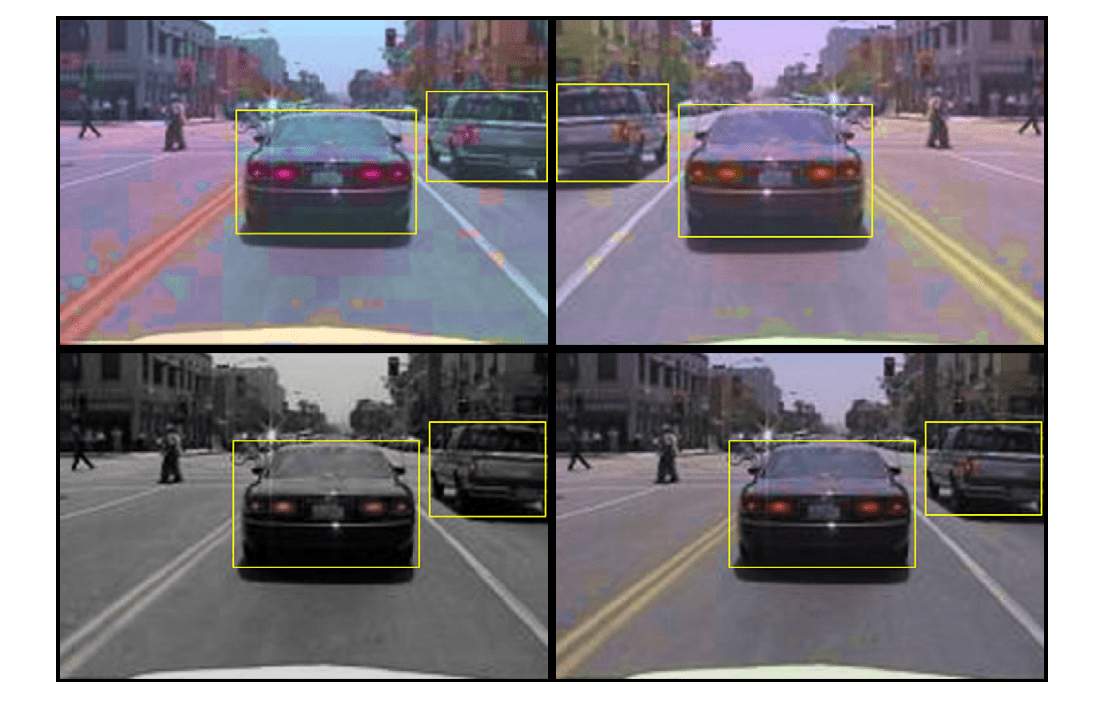
対話形式によるパフォーマンスの可視化および評価
Object Detector Analyzer (Computer Vision Toolbox)アプリを使用すると、対話形式で検出器のパフォーマンスをグラウンド トゥルースと比較して可視化し、評価できます。アプリはテスト セットで検出器を実行し、AP や mAP などのメトリクスを計算し、適合率-再現率曲線をプロットし、テスト セット内の各イメージの検出結果を表示します。グラウンド トゥルース データと正解の検出器予測および不正解の検出器予測を並べて可視化し、検出器による誤りが最も多いイメージをすばやく見つけ出して、パフォーマンスをより深く理解できます。アプリを起動するには、objectDetectorAnalyzer 関数を使用します。
objectDetectorAnalyzer(results,testData)
パフォーマンス メトリクスの計算
evaluateObjectDetection (Computer Vision Toolbox)関数を使用し、テスト セットの検出結果に基づいてオブジェクト検出パフォーマンスのメトリクスを計算します。パフォーマンス メトリクスの詳細については、Evaluate Object Detector Performance (Computer Vision Toolbox)を参照してください。
metrics = evaluateObjectDetection(results,testData);
平均適合率 (AP) は、検出器が正しい分類を実行できること (適合率) と検出器がすべての関連オブジェクトを検出できること (再現率) を示す単一の数値です。適合率/再現率 (PR) の曲線は、さまざまなレベルの再現率における検出器の適合率を示しています。すべてのレベルの再現率で適合率が 1 になるのが理想的です。PR 曲線をプロットし、平均適合率も表示します。
[precision,recall] = precisionRecall(metrics);
AP = averagePrecision(metrics);

figure
plot(recall{:},precision{:})
xlabel("Recall")
ylabel("Precision")
grid on
title("Average Precision = "+AP)
YOLO v3 を使用したオブジェクトの検出
学習させた YOLO v3 オブジェクト検出器を使用して、テスト イメージに対して推論を実行します。
テスト データストアを読み取り、サンプル イメージを選択します。
data = read(testData);
I = data{1};
detect (Computer Vision Toolbox)オブジェクト関数を使用して、各オブジェクトのマスク、ラベル、および信頼度スコアを予測します。
[bboxes,scores,labels] = detect(yolov3Detector,I);
insertObjectAnnotation (Computer Vision Toolbox)関数を使用し、イメージに重ねてオブジェクトの注釈を表示します。
I = insertObjectAnnotation(I,"rectangle",bboxes,scores);
figure
imshow(I)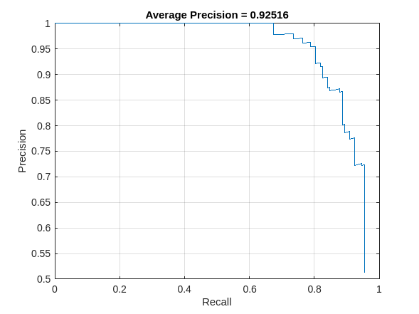
サポート関数
augmentData
function data = augmentData(A)
% Apply random horizontal flipping, and random X/Y scaling. Boxes that get
% scaled outside the bounds are clipped if the overlap is above 0.25. Also,
% jitter image color.

data = cell(size(A));
for ii = 1:size(A,1)
    I = A{ii,1};
    bboxes = A{ii,2};
    labels = A{ii,3};
    sz = size(I);

    if numel(sz) == 3 && sz(3) == 3
        I = jitterColorHSV(I, ...
            Contrast=0, ...
            Hue=0.1, ...
            Saturation=0.2, ...
            Brightness=0.2);
    end

    % Randomly flip image.
    tform = randomAffine2d(XReflection=true,Scale=[1 1.1]);
    rout = affineOutputView(sz,tform,BoundsStyle="centerOutput");
    I = imwarp(I,tform,OutputView=rout);

    % Apply same transform to boxes.
    [bboxes,indices] = bboxwarp(bboxes,tform,rout,OverlapThreshold=0.25);
    bboxes = round(bboxes);
    labels = labels(indices);

    % Return original data only when all boxes are removed by warping.
    if isempty(indices)
        data(ii,:) = A(ii,:);
    else
        data(ii,:) = {I,bboxes,labels};
    end
end
end
preprocessData
function data = preprocessData(data,targetSize)
% Resize the images and scale the pixels to between 0 and 1. Also scale the
% corresponding bounding boxes.

for ii = 1:size(data,1)
    I = data{ii,1};
    imgSize = size(I);

    % Convert an input image with single channel to 3 channels.
    if numel(imgSize) < 3
        I = repmat(I,1,1,3);
    end
    bboxes = data{ii,2};

    I = im2single(imresize(I,targetSize(1:2)));
    scale = targetSize(1:2)./imgSize(1:2);
    bboxes = bboxresize(bboxes,scale);

    data(ii,1:2) = {I,bboxes};
end
end
downloadPretrainedYOLOv3Detector
function detector = downloadPretrainedYOLOv3Detector()
% Download a pretrained yolov3 detector.
if ~exist("yolov3SqueezeNetVehicleExample_21aSPKG.mat","file")
    if ~exist("yolov3SqueezeNetVehicleExample_21aSPKG.zip","file")
        disp("Downloading pretrained detector...");
        pretrainedURL = "https://ssd.mathworks.com/supportfiles/vision/data/yolov3SqueezeNetVehicleExample_21aSPKG.zip";
        websave("yolov3SqueezeNetVehicleExample_21aSPKG.zip",pretrainedURL);
    end
    unzip("yolov3SqueezeNetVehicleExample_21aSPKG.zip");
end
pretrained = load("yolov3SqueezeNetVehicleExample_21aSPKG.mat");
detector = pretrained.detector;
end
参考文献
[1] Redmon, Joseph, and Ali Farhadi. "YOLOv3: An Incremental Improvement." Preprint, submitted April 8, 2018. https://arxiv.org/abs/1804.02767.
参考
アプリ
関数
estimateAnchorBoxes(Computer Vision Toolbox) |analyzeNetwork|combine|transform|read|evaluateObjectDetection(Computer Vision Toolbox)
オブジェクト
boxLabelDatastore(Computer Vision Toolbox) |imageDatastore|dlnetwork|dlarray
トピック
- アンカー ボックスによるオブジェクトの検出 (Computer Vision Toolbox)
- 学習データからのアンカー ボックスの推定 (Computer Vision Toolbox)
- ディープ ネットワーク デザイナーを使用した転移学習用のネットワークの準備
- 深層学習を使用したオブジェクト検出入門 (Computer Vision Toolbox)