2 リンクロボットの LTV モデル

この例では次を使用します。

この例では、所定の軌跡に沿った 2 リンクロボットの LTV モデルを取得する方法を示します。ロボットモデルおよび対応するダイナミクスは [1] および [2] を基にしています。

非線形モデル

次の図に 2 リンク平面ロボットの概略図を示します。

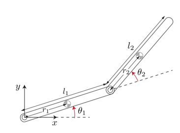
ロボットのコンフィギュレーションは、ジョイント角度 $θ_{1}$ および $θ_{2}$ と先端の位置を制御するジョイントに加えられるトルク $τ_{1}$ および $τ_{2}$ で記述されます。状態ベクトルは次のとおりです。

$x (t) = [\begin{array}{c} θ_{1} \\ θ_{2} \\ {\dot{θ}}_{1} (t) \\ {\dot{θ}}_{2} (t) \end{array}]$ .

ロボットダイナミクスは次の方程式で記述されます。

$[\begin{array}{c} α + 2 β \cos (θ_{2}) & δ + β \cos (θ_{2}) \\ δ + β \cos (θ_{2}) & δ \end{array}] [\begin{array}{c} \ddot{θ_{1}} \\ \ddot{θ_{2}} \end{array}] + [\begin{array}{c} - β \sin (θ_{2}) \dot{θ_{2}} & β \sin (θ_{2}) (\dot{θ_{1}} + \dot{θ_{2}}) \\ β \sin (θ_{2}) \dot{θ_{1}} & 0 \end{array}] [\begin{array}{c} \dot{θ_{1}} \\ \dot{θ_{2}} \end{array}] = [\begin{array}{c} τ_{1} \\ τ_{2} \end{array}]$

ここで、以下となります。

$α = I_{z1} + I_{z2} + m_{1} r_{1}^{2} + m_{2} (l_{1}^{2} + r_{2}^{2})$

$β = m_{2} l_{1} r_{2}$

$δ = I_{z2} + m_{2} r_{2}^{2}$

この例では、この逆運動学問題を twoLinkInverseKinematics.m スクリプトを使用して解きます。

物理パラメーターを定義します。

m1 = 3;         % Mass of link 1, kg
m2 = 2;         % Mass of link 2, kg
L1 = 0.3;       % Length of link 1, meters
L2 = 0.3;       % Length of link 2, meters

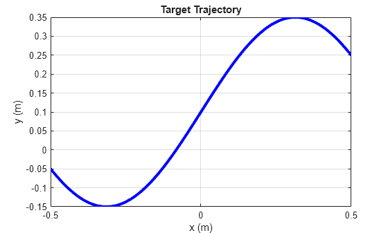
目的の軌跡と逆運動学

アームの先端は所定の平面軌跡 $X (t)$ , $Y (t)$ に従わなければなりません。

T0 = 0;
Tf = 5;
tref = linspace(T0,Tf,400)';
load XYTrajectory x2ref y2ref
plot( x2ref, y2ref, 'b', 'LineWidth',3,'MarkerSize',10)
xlabel('x (m)');
ylabel('y (m)');
grid on
title('Target Trajectory')

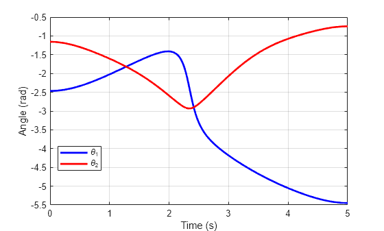
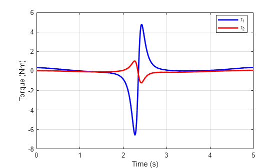
Figure contains an axes object. The axes object with title Target Trajectory, xlabel x (m), ylabel y (m) contains an object of type line.

リンク 2 の終点の運動に対応するジョイント角度、ジョイント速度、およびトルク入力の逆運動学問題を解きます。ジョイント角度を使用してリンク 1 の先端の軌跡を計算します。

[x,tau] = twoLinkInverseKinematics(tref,x2ref,y2ref,m1,m2,L1,L2);
x1ref = L1*cos(x(:,1));
y1ref = L1*sin(x(:,1));

ジョイント角度とトルクをプロットします。

plot(tref,x(:,1),'b',tref,x(:,2),'r','LineWidth',2);
legend('\theta_1','\theta_2','location','Best')
ylabel('Angle (rad)')
xlabel('Time (s)')
grid on;

$Figure contains an axes object. The axes object with xlabel Time (s), ylabel Angle (rad) contains 2 objects of type line. These objects represent \theta_1, \theta_2.$

plot(tref,tau(:,1),'b',tref,tau(:,2),'r','LineWidth',2);
legend('\tau_1','\tau_2','location','Best')
ylabel('Torque (Nm)')
xlabel('Time (s)')
grid on;

$Figure contains an axes object. The axes object with xlabel Time (s), ylabel Torque (Nm) contains 2 objects of type line. These objects represent \tau_1, \tau_2.$

2 リンクロボットの Simscape™ Multibody™ モデルを使用して、計算トルクに対するロボットの応答をシミュレートします。

tau1 = tau(:,1);
tau2 = tau(:,2);
xinit = x(1,:)';  % initial state

open_system('TwoLinkRobotSM')

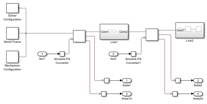
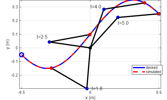
モデルをシミュレートし、結果を展開し、先端が目的の軌跡に従っていることを確認します。

out = sim('TwoLinkRobotSM','ReturnWorkspaceOutputs', 'on');
tsim = out.xsim.time;
xsim = out.xsim.signals.values;

plotTrajectory(xsim,tref,x1ref,y1ref,x2ref,y2ref,L1,L2)

Figure contains an axes object. The axes object with xlabel x (m), ylabel y (m) contains 8 objects of type line, text. One or more of the lines displays its values using only markers These objects represent desired, simulated.

LTV モデル

目的の軌跡に沿った 2 リンクロボットの LTV モデルを作成するために、シミュレーションの開始から終了までの 50 個の等間隔な時間における線形化スナップショットを撮ります。linearize を使用して、対応する操作条件の線形化モデルを取得します。

線形化 I/O を指定します。

io = [...
   linio('TwoLinkRobotSM/tau1',1,'input');...
   linio('TwoLinkRobotSM/tau2',1,'input');...
   linio('TwoLinkRobotSM/Mux',1,'output')];

スナップショットの操作点を取得します。

tlin = linspace(T0,Tf,50);
op = findop('TwoLinkRobotSM',tlin);

オフセットをもつ線形化を計算します。

linOpt = linearizeOptions('StoreOffsets',true);
[G,~,info] = linearize('TwoLinkRobotSM',io,op,linOpt);
G.u = 'tau';
G.y = 'x';
G.SamplingGrid = struct('Time',tlin);

ssInterpolant を使用して、線形化モデルと関連オフセットの配列から LTV オブジェクトを作成します。結果の LTV モデルは、線形化されたダイナミクスをスナップショット時間 tlin の間に内挿します。

Gltv = ssInterpolant(G,info.Offsets);
Gltv.StateName

ans = 4×1 cell
    {'TwoLinkRobotSM.Subsystem.Revolute_Joint1.Rz.q'}
    {'TwoLinkRobotSM.Subsystem.Revolute_Joint1.Rz.w'}
    {'TwoLinkRobotSM.Subsystem.Revolute_Joint2.Rz.q'}
    {'TwoLinkRobotSM.Subsystem.Revolute_Joint2.Rz.w'}

線形化では状態が異なる順序になります。xperm を使用して、状態の順序を $θ_{1}$ 、 $θ_{2}$ 、 ${\dot{θ}}_{1}$ 、 ${\dot{θ}}_{2}$ の順に合わせて並べ替えます。

Gltv = xperm(Gltv,[1 3 2 4]);
Gltv.StateName

ans = 4×1 cell
    {'TwoLinkRobotSM.Subsystem.Revolute_Joint1.Rz.q'}
    {'TwoLinkRobotSM.Subsystem.Revolute_Joint2.Rz.q'}
    {'TwoLinkRobotSM.Subsystem.Revolute_Joint1.Rz.w'}
    {'TwoLinkRobotSM.Subsystem.Revolute_Joint2.Rz.w'}

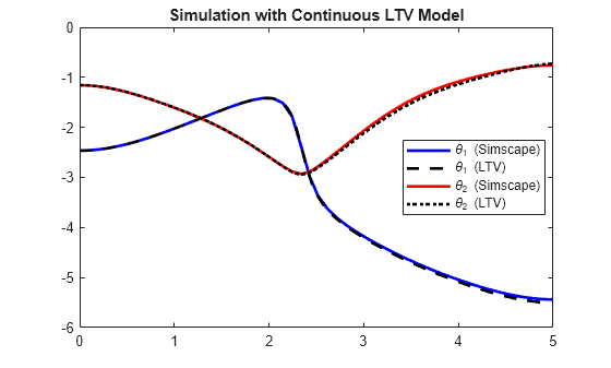
LTV モデルの検証

この LTV モデルの同じトルク入力に対する応答をシミュレートし、Simscape Multibody の結果と比較します。

トルクプロファイルに対する LTV の応答をシミュレートします。

xltv = lsim(Gltv,[tau1 tau2],tref,xinit);

Simscape の結果と比較します。

clf 
plot(tsim,xsim(:,1),'b',tref,xltv(:,1),'k--',...
   tsim,xsim(:,2),'r',tref,xltv(:,2),'k:','LineWidth',2);
xlim([0 5])
legend('\theta_1 (Simscape)','\theta_1 (LTV)',...
   '\theta_2 (Simscape)','\theta_2 (LTV)','location','Best')
title('Simulation with Continuous LTV Model')

$Figure contains an axes object. The axes object with title Simulation with Continuous LTV Model contains 4 objects of type line. These objects represent \theta_1 (Simscape), \theta_1 (LTV), \theta_2 (Simscape), \theta_2 (LTV).$

離散化

組み込みアプリケーションでは、簡単にシミュレートできる離散モデルが必要なことがよくあります。c2d を使用して、Gltv の Tustin 離散化を計算し、それをグリッド付き離散 LTV モデルにすることができます。

Ts = 0.05;
Gd = c2d(Gltv,Ts,'tustin');

Gd を 50 個のグリッド点をもつグリッド付き LTV モデルにします。

k = round(linspace(0,Tf/Ts,50));
Gd = ssInterpolant(Gd,struct('Time',k));

Tustin 離散化の初期条件は次のとおりです。

$z_{0} = x (0) - \frac{T_{s}}{2} \dot{x} (0)$ .

[A,B,~,~,~,dx0,x0,u0] = Gltv.DataFunction(0);
dxinit = dx0+A*(xinit-x0)+B*(tau(1,:)'-u0);
zinit = xinit-Ts/2*dxinit;

シミュレートして Simscape の結果と比較します。

t = T0:Ts:Tf;
taud = interp1(tref,[tau1 tau2],t);
xd = lsim(Gd,taud,t,zinit);

clf 
plot(tsim,xsim(:,1),'b',t,xd(:,1),'k--',...
   tsim,xsim(:,2),'r',t,xd(:,2),'k:','LineWidth',2);
xlim([0 5])
legend('\theta_1 (Simscape)','\theta_1 (discrete LTV)',...
   '\theta_2 (Simscape)','\theta_2 (discrete LTV)','location','Best')
title('Simulation with Discretized LTV Model')

$Figure contains an axes object. The axes object with title Simulation with Discretized LTV Model contains 4 objects of type line. These objects represent \theta_1 (Simscape), \theta_1 (discrete LTV), \theta_2 (Simscape), \theta_2 (discrete LTV).$

参考文献

[1] Murray, Richard M., Zexiang Li, and Shankar Sastry. A Mathematical Introduction to Robotic Manipulation. Boca Raton: CRC Press, 1994.

[2] Seiler, Peter, Robert M. Moore, Chris Meissen, Murat Arcak, and Andrew Packard. “Finite Horizon Robustness Analysis of LTV Systems Using Integral Quadratic Constraints.” Automatica 100 (February 2019): 135–43. https://doi.org/10.1016/j.automatica.2018.11.009.

参考

2 リンク ロボットの LTV モデル