風力タービンの制御設計

この例では次を使用します。

この例では、1.5 MW の風力タービンの制御システムについて説明します。この例では、ドライブトレイン、ブレード、およびタワーの柔軟モードは無視し、回転子のダイナミクスを単純な 1 次システムとしてモデル化します。強風下でのブレードピッチのゲインスケジュールコントローラーの設計と検証に焦点を当てています。詳細については、[1] および [2] を参照してください。

タービンのモデルとデータ

低速回転シャフトの剛体ダイナミクスは次のとおりです。

$J \dot{ω} = T_{a} - T_{g}$ ,

ここで、 $ω$ は回転子速度、 $T_{a}$ は空力トルク、 $T_{g}$ は高速回転シャフトに接続された発電機からの反作用トルクです。

空力トルクは風速とブレードピッチに依存します。その計算には、次で構成される電力係数データが含まれます。

先端速度比 (単位なし) のグリッド TSRgrid。先端速度比は $TSR = \frac{R ω}{V}$ です。ここで、 $R$ は回転子半径 (m)、 $ω$ は回転子速度 (rad/s)、 $V$ は風速 (m/s) です。
ブレードピッチ角 (度) のグリッド Bgrid。
先端速度比とブレードピッチ角のグリッドに対する電力係数 $C_{p}$ (単位なし) のテーブル CpData。タービンによって生成される電力は $0.5 {ρ AV}^{3} C_{p}$ です。ここで、 $ρ$ は空気密度 (kg/m^3)、 $A = π R^{2}$ は回転子領域 (m) です。

このデータは、ブレードピッチと先端速度比の広範な値から生成されたものです。標準操作点は $C_{p} > 0$ に対応します。テーブルには $C_{p} < 0$ のエントリも一部含まれています (それらの点では、実際にはタービンが動作するのにエネルギーが必要になります)。 $C_{p} < 0$ である点は注意して使用してください。

データを読み込みます。

load WindCpData Bgrid TSRgrid CpData

この例で使用するタービンの物理パラメーターの値は次のとおりです。

GBRatio = 88;      % Gearbox ratio, unitless
GBEff = 1.0;       % Gearbox efficiency, unitless (=1 for perfect eff.)
GenEff = 0.95;     % Generator efficiency, unitless (=1 for perfect eff.)
Jgen = 53;         % Generator Inertia about high-speed shaft, kg*m^2
Jrot = 3e6;        % Rotor inertia about low-speed shaft, kg*m^2
Jeq = Jrot+Jgen*GBRatio^2; % Equiv. inertia about low-speed shaft, kg*m^2
R = 35;            % Rotor radius, m
rho = 1.225;       % Air density, kg/m^3
wPA = 8.6;         % Pitch actuator natural frequency, rad/s
zetaPA = 0.8;      % Pitch actuator damping ratio, unitless
Bmax = 90;         % Maximum blade pitch angle, degrees
Kaw = 0.5;         % Anti-windup gain, rad/s/degree

Simulink® モデル WindTurbineOpenLoop は、回転子のダイナミクスの簡略化モデルを実装したものです。モデルを開きます。

open_system('WindTurbineOpenLoop')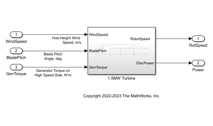

定格操作点と操作領域

風力タービンのパワーエレクトロニクスは、一定の最大電力までしか生成しないようにサイズが調整されています。この最大電力をタービンの "定格電力" と呼びます (このタービンでは 1.5 MW)。トルク、風速、および回転子速度の定格値は、タービンが定格電力を達成する操作条件に対応します。

定格電力を 1.5 MW と指定します。

PRated = 1.5e6;

定格回転子速度は、高速回転シャフト (HSS) では 1800 rpm です。低速回転シャフト (LSS) では、この速度を rad/s に変換します。

wRatedHSS = 1800*(2*pi/60);
wRatedLSS = wRatedHSS/GBRatio;

定格電力は、定格の回転子速度、発電機トルク、および発電機効率の積です。高速回転シャフトの定格発電機トルク (N $\times$ m) を計算します。

GenTRated = PRated/(wRatedHSS*GenEff);

定格風速 (m/s) を指定します。これは、定格回転子速度と定格発電機トルクを達成する風速です。これらの値は平衡点 ( $C_{p} < C_{p, \max}$ のとき) を形成します。

WindRated = 11.2;

定格操作点で区切られる 2 つの操作領域間でコントローラーが切り替わります。

領域 2 (トルク制御): 風速が定格に満たない場合、ブレードピッチは最適 (最高効率) 値に設定され、発電機トルクは $ω^{2}$ に比例する値に設定されます。
領域 3 (ブレードピッチ制御): 風速が定格を超える場合、発電機トルクは定格値に設定されますが、ブレードピッチは定格回転子速度を維持しながら定格電力を供給するように調整されます。

領域 2 の発電機トルクは、GenTRated = Kreg2 $\times$ wRatedLSS^2 に設定されます。ここで、 $Kreg2$ は領域 3 との遷移が滑らかになるように選択します。回転子速度は wRatedLSS、発電機トルクは GenTRated です。

Kreg2 = GenTRated / wRatedLSS^2

Kreg2 = 
1.8257e+03

最後に、最大電力係数および対応する最適な先端速度比とブレードピッチ角を計算します。

CpMax = max(CpData,[],'all');
[i,j] = find(CpData==CpMax);
TSRopt = TSRgrid(i);
Bopt = Bgrid(j);

風速の関数としての最適操作条件

4 ～ 24 m/s の範囲の風速について、最適な定常状態の操作条件を計算します。

平衡点を計算するための風速データを指定し、配列を初期化して LSS の回転子速度、発電機トルク、ブレードピッチ角、および供給電力を格納します。

WindData = sort([4:0.5:24 WindRated]);

nW = numel(WindData);
wLSSeq = zeros(nW,1); 
GenTeq = zeros(nW,1); 
BladePitcheq = zeros(nW,1);
Peq = zeros(nW,1);

領域 2 (トルク制御) では、回転子速度は風速に比例し、ブレードピッチは Bopt に設定されます。

for i=1:nW
    Wind = WindData(i);
    if Wind<=WindRated
        % Region 2: Torque Control
        wLSSeq(i) = Wind/WindRated*wRatedLSS;
        GenTeq(i) = Kreg2*wLSSeq(i)^2;
        wHSS = wLSSeq(i)*GBRatio;
        Peq(i) = GenTeq(i)*wHSS*GenEff; % wRatedHSS*GenEff;
        BladePitcheq(i) = Bopt;
        % Populate operating point
        op(i) = operpoint('WindTurbineOpenLoop');
        op(i).States.x = wLSSeq(i);
        op(i).Inputs(1).u = Wind;
        op(i).Inputs(2).u = BladePitcheq(i);
        op(i).Inputs(3).u = GenTeq(i);
    end
end

領域 3 (ブレードピッチ制御) では、回転子速度と発電機トルクが定格値の wRatedLSS と GenTRated, respectively に達します。findop を使用して、それらの定常値を維持するブレードピッチ角を計算します。

平衡化オプションを指定します。

opt = findopOptions('DisplayReport','off', 'OptimizerType','lsqnonlin');
opt.OptimizationOptions.Algorithm = 'trust-region-reflective';

バッチ平衡化を実行します。

opspec = operspec('WindTurbineOpenLoop');
for i=1:nW
    Wind = WindData(i);
    if Wind>WindRated
        % Region 3: Blade Pitch Control
        wLSSeq(i) = wRatedLSS;
        GenTeq(i) = GenTRated;
        Peq(i) = PRated;
        % Trim condition
        opspec.States.Known = 1;
        opspec.States.SteadyState = 1;
        opspec.Inputs(1).Known=1;
        opspec.Inputs(1).u = Wind;
        opspec.Inputs(2).min = BladePitcheq(i-1);
        opspec.Inputs(3).Known=1;
        opspec.Inputs(3).u = GenTeq(i);
        % Compute corresponding operating point
        op(i) = findop('WindTurbineOpenLoop',opspec,opt);
        % Log steady-state blade pitch angle
        BladePitcheq(i) = op(i).Inputs(2).u;
    end
end

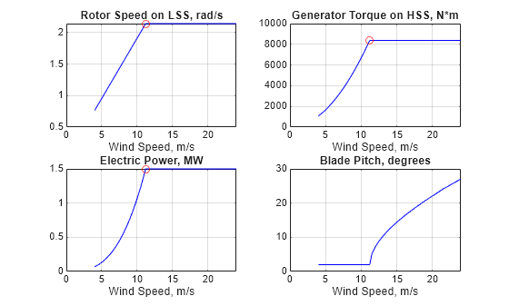
回転子速度、発電機トルク、電力、およびブレードピッチ角の最適な設定を風速の関数としてプロットします。赤い点で定格操作点および領域 2 と 3 の間の遷移をマークします。

clf
subplot(2,2,1)
plot(WindData,wLSSeq,'b',WindRated,wRatedLSS,'ro')
grid on
xlabel('Wind Speed, m/s')
title('Rotor Speed on LSS, rad/s')

subplot(2,2,2)
plot(WindData,GenTeq,'b',WindRated,GenTRated,'ro')
grid on
xlabel('Wind Speed, m/s')
title('Generator Torque on HSS, N*m')

subplot(2,2,3)
plot(WindData,Peq/1e6,'b',WindRated,PRated/1e6,'ro')
grid on
xlabel('Wind Speed, m/s')
title('Electric Power, MW')

subplot(2,2,4)
plot(WindData,BladePitcheq,'b')
grid on
xlabel('Wind Speed, m/s')
title('Blade Pitch, degrees')

バッチ線形化と LPV モデル

前のセクションの操作点について、オフセットを使用して線形化モデルを取得します。

線形化の入力ポイントと出力ポイントを指定します。

io = [linio('WindTurbineOpenLoop/WindSpeed',1,'in');
    linio('WindTurbineOpenLoop/BladePitch',1,'in');
    linio('WindTurbineOpenLoop/GenTorque',1,'in');
    linio('WindTurbineOpenLoop/1.5MW Turbine',1,'out'); % RotorSpeed
    linio('WindTurbineOpenLoop/1.5MW Turbine',2,'out')]; % Power

それぞれの平衡化条件でモデルを線形化します。線形化のオフセット情報を保存するには、info 構造体を出力引数として使用します。

linOpt = linearizeOptions('StoreOffsets',true);
[G,~,info] = linearize('WindTurbineOpenLoop',op,io,linOpt);
G.u = {'WindSpeed'; 'BladePitch'; 'GenTorque'};
G.y = {'RotorSpeed','Power'};
G.SamplingGrid = struct('WindSpeed',WindData);

ssInterpolant を使用して、これらの線形化されたモデルをグリッド点 (風速) 間に内挿する LPV モデルを作成します。

offsets = info.Offsets;
Glpv = ssInterpolant(G,offsets);

固定の風速についての線形解析

風速を定格より下 (領域 2) と定格より上 (領域 3) に分けます。それらの風速におけるタービンの LPV モデルをサンプリングします。

[GR2,GR2offsets] = sample(Glpv,[],WindData( WindData<=WindRated ));
[GR3,GR3offsets] = sample(Glpv,[],WindData( WindData>=WindRated ));

ブレードピッチから回転子速度への線形化のボード応答をプロットします。

clf
bode(GR2(1,2,:),'b',GR3(1,2,:),'r-.')
legend('Region 2','Region 3','Location','Best')
grid on

MATLAB figure

ブレードピッチのゲインスケジュールコントローラー

領域 3 のブレードピッチを調整するためのゲインスケジュール PI コントローラーを設計します。ゲインは、風速よりも確実に測定できるブレードピッチ角でスケジュールされます。ブレードピッチは回転子速度、発電機トルク、および電力が定格値を超えないように調整しなければならないことを思い出してください。

11.5 ～ 24 の間の 20 個の風速の値について、LPV プラントをサンプリングします。

WindGS = linspace(11.5,24,20)';
BladePitchGS = interp1(WindData,BladePitcheq,WindGS);
GGS = sample(Glpv,[],WindGS);

それぞれの風速について、帯域幅 0.66 rad/s を達成するように PI ゲインを調整します。

wL = 0.66;      
opt = pidtuneOptions('PhaseMargin',70);
CPI = pidtune(-GGS(1,2),'pi',wL,opt);
Kp = CPI.Kp(:);
Ki = CPI.Ki(:);

ゲインスケジュールをブレードピッチ角の全範囲に拡張します。

KpGS = [Kp(1); Kp; Kp(end)];
KiGS = [Ki(1); Ki; Ki(end)];
BladePitchGS = [0; BladePitchGS; Bmax];

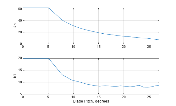
ゲインスケジュールをブレードピッチ角の関数としてプロットします。

clf
subplot(2,1,1)
plot(BladePitchGS,KpGS)
ylabel('Kp')
grid on
xlim(BladePitchGS([1 end-1]))
subplot(2,1,2)
plot(BladePitchGS,KiGS)
ylabel('Ki')
grid on
xlim(BladePitchGS([1 end-1]))
xlabel('Blade Pitch, degrees')

Figure contains 2 axes objects. Axes object 1 with ylabel Kp contains an object of type line. Axes object 2 with xlabel Blade Pitch, degrees, ylabel Ki contains an object of type line.

閉ループの非線形シミュレーション

Simulink モデル WindTurbineClosedLoop は、タービンモデル、領域 2 のトルク制御、および領域 3 のブレードピッチのゲインスケジュール PI コントローラーを組み合わせたものです。

open_system('WindTurbineClosedLoop')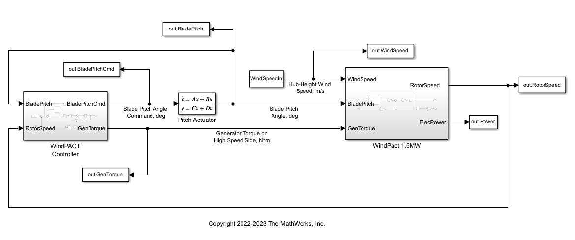

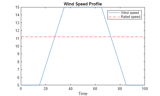
次の風速プロファイルをシミュレーションへの入力として使用します。

V0 = 5;  
Vf = 15;
T1 = 15; 
T2 = 20;  
T3 = 30;   
Tf = 2*T1+2*T2+T3;
WindSpeedIn = [0 V0; T1 V0; T1+T2 Vf; T1+T2+T3 Vf; T1+2*T2+T3 V0; Tf V0];

t = (0:0.1:Tf)';
Wind = interp1(WindSpeedIn(:,1),WindSpeedIn(:,2),t);
clf
plot(t,Wind,[0 Tf],WindRated*[1 1],'r--')
xlabel('Time')
title('Wind Speed Profile')
legend('Wind speed','Rated speed')

Figure contains an axes object. The axes object with title Wind Speed Profile, xlabel Time contains 2 objects of type line. These objects represent Wind speed, Rated speed.

この風プロファイルに対する閉ループ応答を適切な初期条件でシミュレートします。

回転子速度、アクチュエータ状態、および回転子速度誤差の初期条件を指定します。ここでは、V0 < WindRated、つまり領域 2 を想定しています。

w0 = V0/WindRated*wRatedLSS;
xPA0= [Bopt; 0]; 
e0 = wRatedLSS-w0;

コントローラーの積分器が定常状態になる条件を指定します。

0 = e0 + Kaw*(-KpGS(1)*e0-xK0-Bopt)

xK0 = e0*(1/Kaw-KpGS(1))-Bopt;

モデルのシミュレーションを実行します。

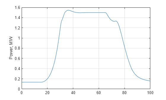
out = sim('WindTurbineClosedLoop',Tf);

電力出力をプロットします。

Power = out.Power;
clf
plot(Power.Time,Power.Data/1e6)
ylabel('Power, MW')
grid on

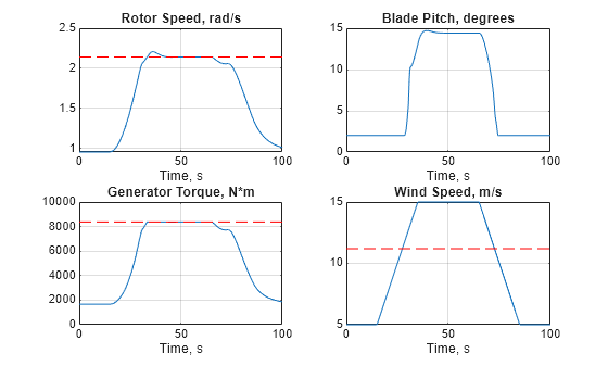
Figure contains an axes object. The axes object with ylabel Power, MW contains an object of type line.

その他の変数をプロットします。

clf
subplot(2,2,1)
RotorSpeed = out.RotorSpeed;
plot(RotorSpeed.Time,RotorSpeed.Data,[0 Tf],wRatedLSS*[1 1],'r--')
title('Rotor Speed, rad/s') 
xlabel('Time, s')
grid on

subplot(2,2,2)
BladePitch = out.BladePitch;
plot(BladePitch.Time,BladePitch.Data);
title('Blade Pitch, degrees'); 
xlabel('Time, s')
grid on

subplot(2,2,3)
GenTorque = out.GenTorque;
plot(GenTorque.Time,GenTorque.Data,[0 Tf],GenTRated*[1 1],'r--')
title('Generator Torque, N*m')
xlabel('Time, s')
grid on;

subplot(2,2,4)
WindSpeed = out.WindSpeed;
plot(WindSpeed.Time,WindSpeed.Data,[0 Tf],WindRated*[1 1],'r--')
title('Wind Speed, m/s') 
xlabel('Time, s')
grid on

閉ループの LPV シミュレーション

さらに、タービンの LPV モデル Glpv と PI ゲインスケジュールから閉ループ LPV モデルを作成し、それを使用して領域 3 のゲインスケジュールコントローラーを検証できます。最初に、ssInterpolant を使用してゲインスケジュールコントローラーの LPV モデルを作成します。

CPI = ss(0,permute(KiGS,[2 3 1]),1,permute(KpGS,[2 3 1]));
CPI.SamplingGrid = struct('BladePitch',BladePitchGS);

Clpv = ssInterpolant(CPI);
Clpv.InputName = 'RotSpeedErr';
Clpv.OutputName = 'BladePitchCmd';
Clpv.StateName = 'Controller';

ブレードピッチのアクチュエータは 2 次システムとしてモデル化されます。

Actuator = ss([0 1; -wPA^2 -2*zetaPA*wPA],[0; wPA^2],[1 0],0);
Actuator.InputName = 'BladePitchCmd';
Actuator.OutputName = 'BladePitch';
Actuator.StateName = {'BladePitch','Act2'};

connect を使用して、LPV プラントとゲインスケジュール PI コントローラーを含む閉ループ LPV モデル Tlpv を作成します。この閉ループモデルは、風速とブレードピッチ角の 2 つのパラメーターに依存します。

SumBlk = sumblk('RotSpeedErr = RotorSpeed - RotSpeedCmd');

Tlpv = connect(Glpv,Clpv,Actuator,SumBlk,...
   {'WindSpeed','RotSpeedCmd','GenTorque'},...
   {'RotorSpeed','Power','BladePitch'});

Tlpv.ParameterName

ans = 2×1 cell
    {'WindSpeed' }
    {'BladePitch'}

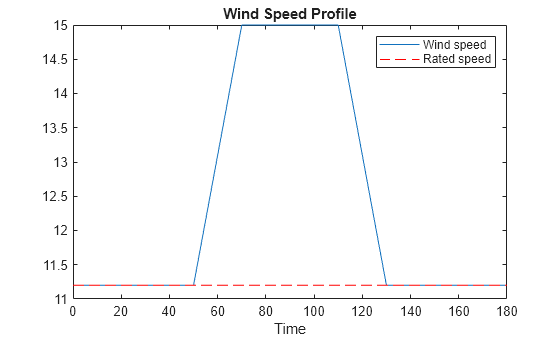
ブレードピッチのコントローラーを検証するために、領域 3 に完全に収まる風プロファイルを使用します。

V0 = WindRated;  
Vf = 15;
T1 = 50;  
T2 = 20;  
T3 = 40;  
Tf = 2*T1+2*T2+T3;
WindSpeedIn = [0 V0; T1 V0; T1+T2 Vf; T1+T2+T3 Vf; T1+2*T2+T3 V0; Tf V0];

t = (0:0.1:Tf)';
Wind = interp1(WindSpeedIn(:,1),WindSpeedIn(:,2),t);
clf 
plot(t,Wind,[0 Tf],WindRated*[1 1],'r--')
xlabel('Time') 
title('Wind Speed Profile')
legend('Wind speed','Rated speed')

Figure contains an axes object. The axes object with title Wind Speed Profile, xlabel Time contains 2 objects of type line. These objects represent Wind speed, Rated speed.

lsim を使用して閉ループ応答をシミュレートします。パラメーターの軌跡を暗黙的に定義します (風速は最初の入力、ブレードピッチ角はアクチュエータモデルの最初の状態です)。

% Inputs
u = zeros(numel(t),3);
u(:,1) = Wind;       % Wind profile
u(:,2) = wRatedLSS;  % Rotor speed
u(:,3) = GenTRated;  % Generator torque

% Initial condition
xinit = [wRatedLSS;Bopt;Bopt;0];

% Parameter trajectory
pFcn = @(t,x,u) [u(1);x(3)];  % x(3) = BladePitch

% LPV simulation
ylpv = lsim(Tlpv,u,t,xinit,pFcn);

同じ風プロファイルについて、非線形シミュレーションを実行します。

w0 = wRatedLSS;  % Initial rotor speed, rad/s
xPA0 = [Bopt; 0];    % Initial actuator state
xK0 = -Bopt;        % integrator output
out = sim('WindTurbineClosedLoop',Tf);

LPV と非線形のシミュレーションを比較します。

RotorSpeed = out.RotorSpeed;
clf
subplot(3,1,1)
plot(RotorSpeed.Time,RotorSpeed.Data,t,ylpv(:,1),'--')
title('Rotor Speed, rad/s')
grid on
Power = out.Power;
subplot(3,1,2)
plot(Power.Time,Power.Data/1e6,t,ylpv(:,2)/1e6,'--')
title('Power, MW')
grid on
BladePitch = out.BladePitch;
subplot(3,1,3)
plot(BladePitch.Time,BladePitch.Data,t,ylpv(:,3),'--')
title('Blade Pitch, Degrees')
grid on
legend('Nonlinear','LPV','location','Best')

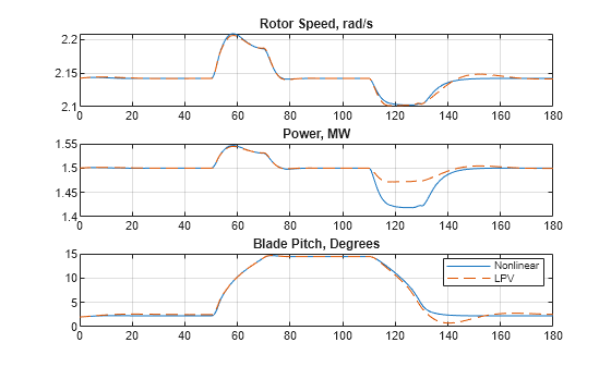
Figure contains 3 axes objects. Axes object 1 with title Rotor Speed, rad/s contains 2 objects of type line. Axes object 2 with title Power, MW contains 2 objects of type line. Axes object 3 with title Blade Pitch, Degrees contains 2 objects of type line. These objects represent Nonlinear, LPV.

LPV シミュレーションでは、回転子速度とブレードピッチは正確にモデル化されていますが、風速が低下したときの電力の低下が低く見積もられています。これは、LPV シミュレーションでは関係 GenTRated = Kreg2 $\times$ wRatedLSS^2 による発電機トルクの低下が考慮されないためです。

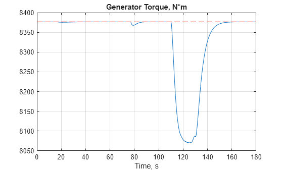
代わりに、発電機トルクを定格値に固定する u(:,3) = GenTRated を設定します。

GenTorque = out.GenTorque;
clf
plot(GenTorque.Time,GenTorque.Data,[0 Tf],GenTRated*[1 1],'r--')
title('Generator Torque, N*m')
xlabel('Time, s')
grid on

Figure contains an axes object. The axes object with title Generator Torque, N*m, xlabel Time, s contains 2 objects of type line.

精度を高めるために、回転子速度データと前述の関係を使用して発電機トルクのデータを推定します。

GenTorque = Kreg2 * ylpv(:,1).^2;
u(:,3) = min(GenTorque,GenTRated);
ylpv = lsim(Tlpv,u,t,xinit,pFcn);

応答をプロットします。

clf
RotorSpeed = out.RotorSpeed;
subplot(3,1,1)
plot(RotorSpeed.Time,RotorSpeed.Data,t,ylpv(:,1),'--')
title('Rotor Speed, rad/s')
grid on
Power = out.Power;
subplot(3,1,2)
plot(Power.Time,Power.Data/1e6,t,ylpv(:,2)/1e6,'--')
title('Power, MW')
grid on
BladePitch = out.BladePitch;
subplot(3,1,3)
plot(BladePitch.Time,BladePitch.Data,t,ylpv(:,3),'--')
title('Blade Pitch, Degrees')
grid on
legend('Nonlinear','LPV','location','Best')

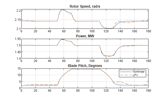
LPV シミュレーションが非線形の内容とほぼ一致します。

参考文献

[1] Malcolm, D.J. and A.C. Hansen. “WindPACT Turbine Rotor Design Study: June 2000–June 2002 (Revised).” National Renewable Energy Laboratory, 2006 NREL/SR-500-32495. https://www.nrel.gov/docs/fy06osti/32495.pdf.

[2] Rinker, Jennifer and Dykes, Katherine. "WindPACT Reference Wind Turbines." National Renewable Energy Laboratory, 2018 NREL/TP-5000-67667. https://www.nrel.gov/docs/fy18osti/67667.pdf.

参考

ssInterpolant | sample | linearize (Simulink Control Design) | ndgrid