rocmetrics
Receiver operating characteristic (ROC) curve and performance metrics for binary and multiclass classifiers
Since R2022a
Description
Create a rocmetrics object to evaluate the performance of a classification model using receiver operating characteristic (ROC) curves or other performance metrics. rocmetrics supports both binary and multiclass problems.
For each class, rocmetrics computes performance metrics for a one-versus-all ROC curve. You can compute metrics for an average ROC curve by
using the average function. After
computing metrics for ROC curves, you can plot them by using the plot function.
By default, rocmetrics computes the false positive rates (FPR) and the true
positive rates (TPR) to obtain a ROC curve. You can compute additional metrics by specifying
the AdditionalMetrics
name-value argument when you create an object or by calling the addMetrics function
after you create an object. A rocmetrics object stores the computed metrics
in the Metrics
properties.
In R2024b: You can find the area under the ROC curve (AUC) using the auc function.
rocmetrics computes pointwise confidence intervals for the performance
metrics when you set the NumBootstraps value to
a positive integer or when you specify cross-validated data for the true class labels
(Labels), classification
scores (Scores), and
observation weights (Weights). For details,
see Pointwise Confidence Intervals.
Creation
Syntax
Description
rocObj = rocmetrics(Labels,Scores,ClassNames)rocmetrics object using the true class labels in
Labels and the classification scores in
Scores. Specify Labels as a vector of length n,
and specify Scores as a matrix of size
n-by-K, where n is the number
of observations, and K is the number of classes.
ClassNames specifies the column order in
Scores.
The Metrics property
contains the performance metrics for each class for which you specify
Scores and ClassNames.
If you specify cross-validated data in Labels and
Scores as cell arrays, then rocmetrics computes
confidence intervals for the performance metrics.
rocObj = rocmetrics(Mdl,Tbl,ResponseVarName)rocmetrics object from a classification model object
Mdl, using the predictor data in Tbl with the
response variable name ResponseVarName as one column in
Tbl.
rocObj = rocmetrics(___,Name=Value)NumBootstraps=100 draws 100 bootstrap samples to compute
confidence intervals for the performance metrics.
Input Arguments
Name-Value Arguments
Properties
Object Functions
addMetrics | Compute additional classification performance metrics |
auc | Area under ROC curve or precision-recall curve |
average | Compute performance metrics for average receiver operating characteristic (ROC) curve in multiclass problem |
modelOperatingPoint | Operating point of rocmetrics object |
plot | Plot receiver operating characteristic (ROC) curves and other performance curves |
Examples
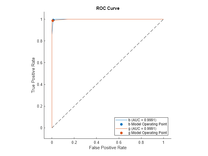
Compute the performance metrics (FPR and TPR) for a binary classification problem by creating a rocmetrics object, and plot a ROC curve by using the plot function.
Load the ionosphere data set. This data set has 34 predictors (X) and 351 binary responses (Y) for radar returns, either bad ('b') or good ('g').
load ionospherePartition the data into training and test sets. Use approximately 80% of the observations to train a support vector machine (SVM) model, and 20% of the observations to test the performance of the trained model on new data. Partition the data using cvpartition.
rng("default") % For reproducibility of the partition
c = cvpartition(Y,Holdout=0.20);
trainingIndices = training(c); % Indices for the training set
testIndices = test(c); % Indices for the test set
XTrain = X(trainingIndices,:);
YTrain = Y(trainingIndices);
XTest = X(testIndices,:);
YTest = Y(testIndices);
Train an SVM classification model.
Mdl = fitcsvm(XTrain,YTrain);
Compute the classification scores for the test set.
[~,Scores] = predict(Mdl,XTest);
size(Scores)
ans = 1×2

    70     2
The output Scores is a matrix of size 70-by-2. The column order of Scores follows the class order in Mdl. Display the class order stored in Mdl.ClassNames.
Mdl.ClassNames
ans = 2×1 cell
    {'b'}
    {'g'}
Create a rocmetrics object by using the true labels in YTest and the classification scores in Scores. Specify the column order of Scores using Mdl.ClassNames.
rocObj = rocmetrics(YTest,Scores,Mdl.ClassNames);
rocObj is a rocmetrics object that stores the performance metrics for each class in the Metrics property. Compute the AUC values using the auc function.
a = auc(rocObj)
a = 1×2

    0.8587    0.8587
For a binary classification problem, the AUC values are equal to each other.
The table in Metrics contains the performance metric values for both classes, vertically concatenated according to the class order. Find the rows for the first class in the table, and display the first eight rows.
idx = strcmp(rocObj.Metrics.ClassName,Mdl.ClassNames(1));
head(rocObj.Metrics(idx,:))
    ClassName    Threshold    FalsePositiveRate    TruePositiveRate
    _________    _________    _________________    ________________

      {'b'}       15.545              0                     0
      {'b'}       15.545              0                  0.04
      {'b'}       15.105              0                  0.08
      {'b'}       11.424              0                  0.16
      {'b'}       10.077              0                   0.2
      {'b'}       9.9716              0                  0.24
      {'b'}       9.9417              0                  0.28
      {'b'}       9.0338              0                  0.32
Plot the ROC curve for each class by using the plot function.
plot(rocObj)

For each class, the plot function plots a ROC curve and displays a filled circle marker at the model operating point. The legend displays the class name and AUC value for each curve.
Note that you do not need to examine ROC curves for both classes in a binary classification problem. The two ROC curves are symmetric, and the AUC values are identical. A TPR of one class is a true negative rate (TNR) of the other class, and TNR is 1-FPR. Therefore, a plot of TPR versus FPR for one class is the same as a plot of 1-FPR versus 1-TPR for the other class.
Plot the ROC curve for the first class only by specifying the ClassNames name-value argument.
plot(rocObj,ClassNames=Mdl.ClassNames(1))

Compute the performance metrics (FPR and TPR) for a multiclass classification problem by creating a rocmetrics object, and plot a ROC curve for each class by using the plot function. Specify the AverageCurveType name-value argument of plot to create the average ROC curve for the multiclass problem.
Load the fisheriris data set. The matrix meas contains flower measurements for 150 different flowers. The vector species lists the species for each flower. species contains three distinct flower names.
load fisheririsTrain a classification tree that classifies observations into one of the three labels. Cross-validate the model using 10-fold cross-validation.
rng("default") % For reproducibility
Mdl = fitctree(meas,species,Crossval="on");
Compute the classification scores for validation-fold observations.
[~,Scores] = kfoldPredict(Mdl);
size(Scores)
ans = 1×2

   150     3
The output Scores is a matrix of size 150-by-3. The column order of Scores follows the class order in Mdl. Display the class order stored in Mdl.ClassNames.
Mdl.ClassNames
ans = 3×1 cell
    {'setosa'    }
    {'versicolor'}
    {'virginica' }
Create a rocmetrics object by using the true labels in species and the classification scores in Scores. Specify the column order of Scores using Mdl.ClassNames.
rocObj = rocmetrics(species,Scores,Mdl.ClassNames);
rocObj is a rocmetrics object that stores the performance metrics for each class in the Metrics property. Compute the AUC values by using the auc function.
a = auc(rocObj)
a = 1×3

    1.0000    0.9636    0.9636
The table in Metrics contains the performance metric values for all three classes, vertically concatenated according to the class order. Find and display the rows for the second class in the table.
idx = strcmp(rocObj.Metrics.ClassName,Mdl.ClassNames(2));
rocObj.Metrics(idx,:)
ans=13×4 table
      ClassName       Threshold    FalsePositiveRate    TruePositiveRate
    ______________    _________    _________________    ________________

    {'versicolor'}           1              0                    0
    {'versicolor'}           1           0.01                  0.7
    {'versicolor'}     0.95455           0.02                  0.8
    {'versicolor'}     0.91304           0.03                  0.9
    {'versicolor'}        -0.2           0.04                  0.9
    {'versicolor'}    -0.33333           0.06                  0.9
    {'versicolor'}        -0.6           0.08                  0.9
    {'versicolor'}    -0.86957           0.12                 0.92
    {'versicolor'}    -0.91111           0.16                 0.96
    {'versicolor'}    -0.95122           0.31                 0.96
    {'versicolor'}    -0.95238           0.38                 0.98
    {'versicolor'}    -0.95349           0.44                 0.98
    {'versicolor'}          -1              1                    1
Plot the ROC curve for each class. Specify AverageCurveType="micro" to compute the performance metrics for the average ROC curve using the micro-averaging method.
plot(rocObj,AverageCurveType="micro")
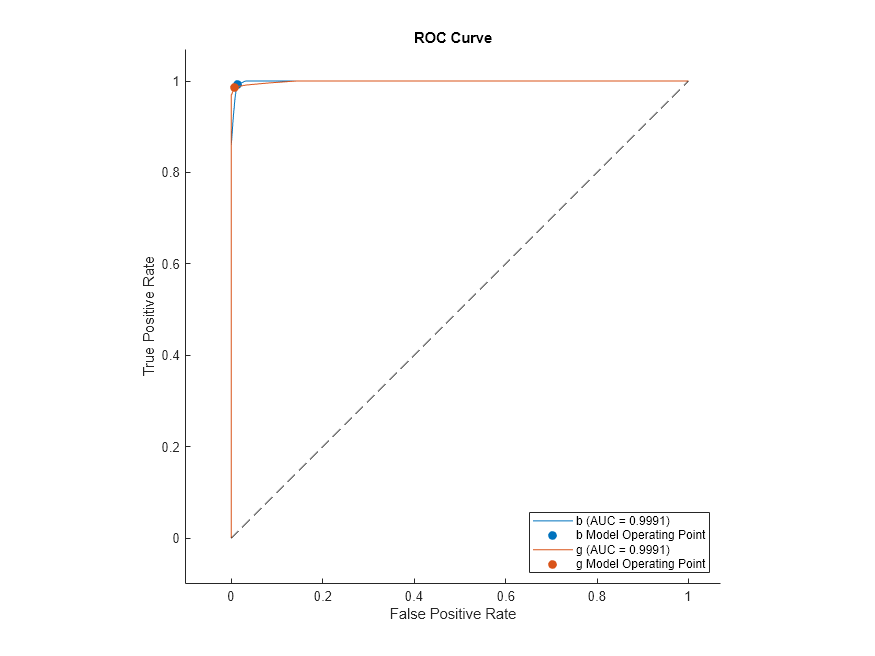
Load the ionosphere data into your workspace.
load ionosphere
who
Your variables are: Description X Y
The data is in variable X and the response is in variable Y. Create a classification tree model of the data.
Mdl = fitctree(X,Y);
Create rocmetrics Object from Model and Matrix Data
Create a rocmetrics object from the classification tree model, using X and Y as the predictor data and response data.
rocMdl = rocmetrics(Mdl,X,Y);
Plot the ROC curve for the rocmetrics object.
plot(rocMdl)
Create rocmetrics Object from Model and Table Data
Create a table of the X data.
save("datafile.txt","X","-ascii");
Tbl = readtable("datafile.txt");
Create a rocmetrics object from the classification tree model, using Tbl as the predictor data and Y as the response data.
Mdl2 = fitctree(Tbl,Y);
rocMdl2 = rocmetrics(Mdl2,Tbl,Y);
Plot the ROC curve for rocMdl2. The plot is the same as the previous one.
plot(rocMdl2)
Create rocmetrics Object from Model and Table with Response
Place the response data Y into Tbl with the variable name Resp.
Tbl.Resp = Y;
Create a rocmetrics object from Tbl specifying Resp as the response variable name.
Mdl3 = fitctree(Tbl,"Resp");
rocMdl3 = rocmetrics(Mdl3,Tbl,"Resp");
Plot the ROC curve for rocMdl3. The plot is the same as the previous ones.
plot(rocMdl3)
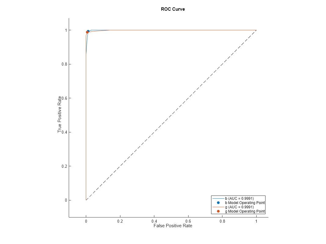
Create rocmetrics Object from Cross-Validated Model
Create a cross-validated classification tree model.
rng default % For reproducibility
CVMdl = fitctree(X,Y,KFold=5);
Create a rocmetrics object from the cross-validated model.
rocMdl4 = rocmetrics(CVMdl);
Plot the ROC curve for rocMdl4.
plot(rocMdl4)
This ROC curve looks different than the previous ones. The cross-validated model has more realistic ROC curves.
k-nearest neighbor (KNN), discriminant analysis, and naive Bayes classifiers use expected classification costs rather than scores to predict labels. When you want to use nondefault misclassification costs to create ROC curves for these models, set the ApplyCostToScores name-value argument of the rocmetrics function to true.
Read the sample file CreditRating_Historical.dat into a table. The predictor data consists of financial ratios and industry sector information for a list of corporate customers. The response variable consists of credit ratings assigned by a rating agency.
creditrating = readtable("CreditRating_Historical.dat");Because each value in the ID variable is a unique customer ID, that is, length(unique(creditrating.ID)) is equal to the number of observations in creditrating, the ID variable is a poor predictor. Remove the ID variable from the table.
creditrating = removevars(creditrating,"ID");Combine all the A ratings into one rating. Do the same for the B and C ratings, so that the response variable has three distinct ratings. Among the three ratings, A is considered the best and C the worst.
Rating = categorical(creditrating.Rating);
Rating = mergecats(Rating,["AAA","AA","A"],"A");
Rating = mergecats(Rating,["BBB","BB","B"],"B");
Rating = mergecats(Rating,["CCC","CC","C"],"C");
creditrating.Rating = Rating;
Assume that specific costs are associated with misclassifying the credit ratings of customers. Create a matrix variable that contains the misclassification costs. Create another variable that specifies the class names and their order in the matrix variable.
classificationCosts = [0 100 200; 500 0 100; 1000 500 0];
classNames = categorical(["A","B","C"]);
The costs indicate that classifying a customer with bad credit as a customer with good credit is more costly than classifying a customer with good credit as a customer with bad credit. For example, the cost of misclassifying a C rating customer as an A rating customer is $1000.
Partition the data into training and test sets. Use 75% of the observations to train a discriminant analysis classifier, and 25% of the observations to test the performance of the trained model on new data.
rng("default") % For reproducibility
c = cvpartition(creditrating.Rating,"Holdout",0.25);
trainRatings = creditrating(training(c),:);
testRatings = creditrating(test(c),:);
Train a discriminant analysis classifier. Specify the misclassification costs.
mdl = fitcdiscr(trainRatings,"Rating",Cost=classificationCosts, ...
    ClassNames=classNames);
Predict the class labels, scores, and expected classification costs for the observations in the test set.
[labels,scores,expectedCosts] = predict(mdl,testRatings);
For each observation, the predicted class label corresponds to the minimum expected classification cost among all classes rather than the greatest score (or posterior probability).
For example, display the predictions for the first observation in the test set.
firstLabel = labels(1)
firstLabel = categorical
     B
firstScores = array2table(scores(1,:),VariableNames=["A","B","C"])
firstScores=1×3 table
       A          B           C
    _______    _______    __________

    0.70807    0.29193    4.7141e-13
firstExpectedCosts = array2table(expectedCosts(1,:), ...
    VariableNames=["A","B","C"])
firstExpectedCosts=1×3 table
      A         B         C
    ______    ______    ______

    145.96    70.807    170.81
The predicted label corresponds to class B, which has the lowest expected classification cost, even though class A has the greatest posterior probability.
Create a rocmetrics object by using the true labels in testRatings and the classification scores in scores. Specify the column order of scores. To use nondefault misclassification costs and scores returned by a discriminant analysis model, specify the Cost and ApplyCostToScores name-value arguments.
roc = rocmetrics(testRatings.Rating,scores,classNames, ...
    Cost=classificationCosts,ApplyCostToScores=true);
Notice that the scores stored in rocmetrics are the negative expected classification costs.
isequal(roc.Scores,-expectedCosts)
ans = logical
   1
Plot the ROC curve for each class by using the plot function.
plot(roc,ClassNames=classNames)

For each class, the plot function plots a curve. The filled circle markers indicate the model operating points.
Train a cross-validated discriminant analysis classifier by using the entire creditrating data set.
cvmdl = fitcdiscr(creditrating,"Rating",Cost=classificationCosts, ...
    ClassNames=classNames,CrossVal="on")
cvmdl =
  ClassificationPartitionedModel
    CrossValidatedModel: 'Discriminant'
         PredictorNames: {'WC_TA'  'RE_TA'  'EBIT_TA'  'MVE_BVTD'  'S_TA'  'Industry'}
           ResponseName: 'Rating'
        NumObservations: 3932
                  KFold: 10
              Partition: [1×1 cvpartition]
             ClassNames: [A    B    C]
         ScoreTransform: 'none'


  Properties, Methods
The fitcdiscr function creates a ClassificationPartitionedModel object of type Discriminant (CrossValidatedModel property value). To create the cross-validated model, the function completes these steps:
Randomly partition the data into 10 sets.
For each set, reserve the set as validation data, and train the model using the other 9 sets.
Store the 10 compact trained models in a 10-by-1 cell vector in the
Trainedproperty of the cross-validated model object.
cvmdl.Trained
ans=10×1 cell array
    {1×1 classreg.learning.classif.CompactClassificationDiscriminant}
    {1×1 classreg.learning.classif.CompactClassificationDiscriminant}
    {1×1 classreg.learning.classif.CompactClassificationDiscriminant}
    {1×1 classreg.learning.classif.CompactClassificationDiscriminant}
    {1×1 classreg.learning.classif.CompactClassificationDiscriminant}
    {1×1 classreg.learning.classif.CompactClassificationDiscriminant}
    {1×1 classreg.learning.classif.CompactClassificationDiscriminant}
    {1×1 classreg.learning.classif.CompactClassificationDiscriminant}
    {1×1 classreg.learning.classif.CompactClassificationDiscriminant}
    {1×1 classreg.learning.classif.CompactClassificationDiscriminant}
Predict the class label, scores, and expected classification costs for each observation.
[cvlabels,cvscores,cvexpectedCosts] = kfoldPredict(cvmdl);
Plot the ROC curve for each class.
cvroc = rocmetrics(creditrating.Rating,cvscores,classNames, ...
    Cost=classificationCosts,ApplyCostToScores=true);
plot(cvroc,ClassNames=classNames)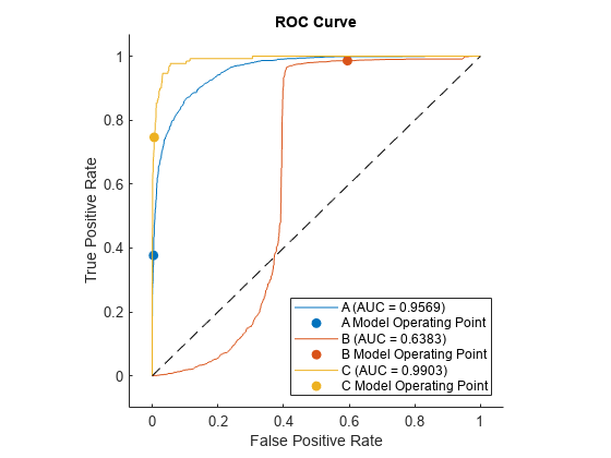
The cross-validation results are similar to the previous test set results.
For generated samples containing outliers, train an isolation forest model and compute anomaly scores by using the iforest function. iforest returns scores as a vector. Use the scores to create a rocmetrics object. Plot the precision-recall curve using the anomaly scores, and find the model operating point for the isolation forest model.
Use a Gaussian copula to generate random data points from a bivariate distribution.
rng("default")
rho = [1,0.05;0.05,1];
n = 1000;
u = copularnd("Gaussian",rho,n);
Add noise to 5% of randomly selected observations to make the observations outliers.
noise = randperm(n,0.05*n);
true_tf = false(n,1);
true_tf(noise) = true;
u(true_tf,1) = u(true_tf,1)*5;
Train an isolation forest model by using the iforest function. Specify the fraction of anomalies in the training observations as 0.05.
[f,tf,scores] = iforest(u,ContaminationFraction=0.05);
f is an IsolationForest object. iforest also returns the anomaly indicators (tf) and anomaly scores (scores) for the training data. iforest determines the threshold value (f.ScoreThreshold) so that the function detects the specified fraction of training observations as anomalies.
Check the performance of the IsolationForest object by plotting the precision-recall curve, which computes the area under the curve (AUC) value. Create a rocmetrics object by using the true anomaly indicators (true_tf) and anomaly scores (scores). A score value close to 1 indicates an anomaly, as does the value true in true_tf. Therefore, specify the class name for scores as true. Specify the AdditionalMetrics name-value argument to compute the precision values (or positive predictive values).
rocObj = rocmetrics(true_tf,scores,true,AdditionalMetrics="PositivePredictiveValue");Plot the curve by using the plot function of rocmetrics. Specify the y-axis metric as precision (or positive predictive value) and the x-axis metric as recall (or true positive rate). Display a filled circle at the model operating point corresponding to f.ScoreThreshold.
r = plot(rocObj,YAxisMetric="PositivePredictiveValue",XAxisMetric="TruePositiveRate",...
    ShowModelOperatingPoint=true);

Compute the confidence intervals for FPR and TPR for fixed threshold values by using bootstrap samples, and plot the confidence intervals for TPR on the ROC curve by using the plot function.
Load the ionosphere data set. This data set has 34 predictors (X) and 351 binary responses (Y) for radar returns, either bad ('b') or good ('g').
load ionospherePartition the data into training and test sets. Use approximately 80% of the observations to train a support vector machine (SVM) model, and 20% of the observations to test the performance of the trained model on new data. Partition the data using cvpartition.
rng("default") % For reproducibility of the partition
c = cvpartition(Y,Holdout=0.20);
trainingIndices = training(c); % Indices for the training set
testIndices = test(c); % Indices for the test set
XTrain = X(trainingIndices,:);
YTrain = Y(trainingIndices);
XTest = X(testIndices,:);
YTest = Y(testIndices);
Train an SVM classification model.
Mdl = fitcsvm(XTrain,YTrain);
Compute the classification scores for the test set.
[~,Scores] = predict(Mdl,XTest);
Create a rocmetrics object by using the true labels in YTest and the classification scores in Scores. Specify the column order of Scores using Mdl.ClassNames. Specify NumBootstraps as 100 to use 100 bootstrap samples to compute the confidence intervals.
rocObj = rocmetrics(YTest,Scores,Mdl.ClassNames, ...
    NumBootstraps=100);
Find the rows for the second class in the table of the Metrics property, and display the first eight rows.
idx = strcmp(rocObj.Metrics.ClassName,Mdl.ClassNames(2));
head(rocObj.Metrics(idx,:))
    ClassName    Threshold        FalsePositiveRate                 TruePositiveRate
    _________    _________    __________________________    ________________________________

      {'g'}        7.196         0          0          0           0           0           0
      {'g'}        7.196         0          0          0    0.022222           0    0.093023
      {'g'}       6.2583         0          0          0    0.044444           0     0.11969
      {'g'}       5.5719         0          0          0    0.066667    0.020988     0.16024
      {'g'}       5.5643         0          0          0    0.088889    0.022635     0.18805
      {'g'}       5.4618      0.04          0    0.22222    0.088889    0.022635     0.18805
      {'g'}       5.3667      0.08          0       0.28    0.088889    0.022635     0.18805
      {'g'}       5.1525      0.08          0       0.28     0.11111    0.045035     0.19532
Each row of the table contains the metric value and its confidence intervals for FPR and TPR for a fixed threshold value. The Threshold variable is a column vector, and the FalsePositiveRate and TruePositiveRate variables are three-column matrices. The first column of the matrices corresponds to the metric values, and the second and third columns correspond to the lower and upper bounds, respectively.
Plot the ROC curve and the confidence intervals for TPR. Specify ShowConfidenceIntervals=true to show the confidence intervals, and specify one class to plot by using the ClassNames name-value argument.
plot(rocObj,ShowConfidenceIntervals=true,ClassNames=Mdl.ClassNames(2))
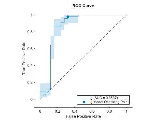
The shaded area around the ROC curve indicates the confidence intervals. The confidence intervals represent the uncertainty of the curve due to the variance in the test set for the trained model.
Compute the confidence intervals for FPR and TPR for fixed threshold values by using cross-validated data, and plot the confidence intervals for TPR on the ROC curve by using the plot function.
Load the fisheriris data set. The matrix meas contains flower measurements for 150 different flowers. The vector species lists the species for each flower. species contains three distinct flower names.
load fisheririsTrain a naive Bayes model that classifies observations into one of the three labels. Cross-validate the model using 10-fold cross-validation.
rng("default") % For reproducibility
Mdl = fitcnb(meas,species,Crossval="on");
Compute the classification scores for validation-fold observations.
[~,Scores] = kfoldPredict(Mdl);
Store the cross-validated scores and the corresponding true labels in cell arrays, so that each element in the cell arrays corresponds to one validation fold.
cv = Mdl.Partition;
numTestSets = cv.NumTestSets;
cvLabels = cell(numTestSets,1);
cvScores = cell(numTestSets,1);
for i = 1:numTestSets
    testIdx = test(cv,i);
    cvLabels{i} = species(testIdx);
    cvScores{i} = Scores(testIdx,:);
end
Create a rocmetrics object using the cell arrays. If you specify true labels and scores by using cell arrays, rocmetrics computes the confidence intervals.
rocObj = rocmetrics(cvLabels,cvScores,Mdl.ClassNames);
Plot the ROC curve and the confidence intervals for TPR. Specify ShowConfidenceIntervals=true to show the confidence intervals.
plot(rocObj,ShowConfidenceIntervals=true)
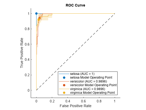
The shaded area around each curve indicates the confidence intervals. The widths of the confidence intervals for setosa are 0 for nonzero false positive rates, so the plot does not have a shaded area for setosa. The confidence intervals reflect the uncertainty in the model due to the variance in the training and test sets.
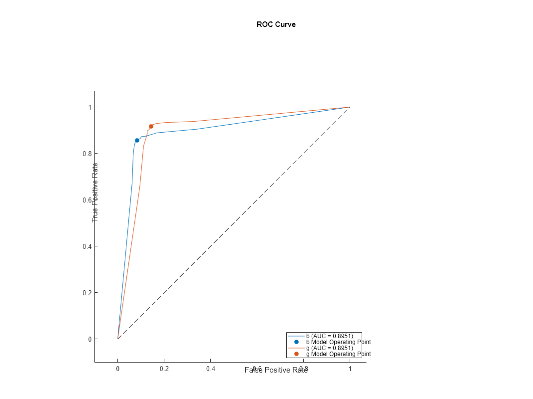
Train three different classification models: decision tree model, generalized additive model, and naive Bayes model. Compare the performance of the three models on a test data set using the ROC curves and the AUC values.
Load the 1994 census data stored in census1994.mat. The data set consists of demographic data from the US Census Bureau to predict whether an individual makes over $50,000 per year.
load census1994census1994 contains the training data set adultdata and the test data set adulttest. Display the unique values in the response variable salary.
classNames = unique(adultdata.salary)
classNames = 2×1 categorical
     <=50K
     >50K
Train the three models by passing the training data adultdata and specifying the response variable name "salary". Specify the order of the classes by using the ClassNames name-value argument.
MdlTree = fitctree(adultdata,"salary",ClassNames=classNames);
MdlGAM = fitcgam(adultdata,"salary",ClassNames=classNames);
MdlNB = fitcnb(adultdata,"salary",ClassNames=classNames);
Compute the classification scores for the test data set adulttest using the trained models.
[~,ScoresTree] = predict(MdlTree,adulttest);
[~,ScoresGAM] = predict(MdlGAM,adulttest);
[~,ScoresNB] = predict(MdlNB,adulttest);
Create a rocmetrics object for each model.
rocTree = rocmetrics(adulttest.salary,ScoresTree,classNames);
rocGAM = rocmetrics(adulttest.salary,ScoresGAM,classNames);
rocNB = rocmetrics(adulttest.salary,ScoresNB,classNames);
Plot the ROC curve for each model. By default, the plot function displays the class names and the AUC values in the legend. To include the model names in the legend instead of the class names, modify the DisplayName property of the ROCCurve object returned by the plot function.
figure
c = cell(3,1);
g = cell(3,1);
[c{1},g{1}] = plot(rocTree,ClassNames=classNames(1));
hold on
[c{2},g{2}] = plot(rocGAM,ClassNames=classNames(1));
[c{3},g{3}] = plot(rocNB,ClassNames=classNames(1));
modelNames = ["Decision Tree Model", ...
    "Generalized Additive Model","Naive Bayes Model"];
for i = 1 : 3
    c{i}.DisplayName = replace(c{i}.DisplayName, ...
        string(classNames(1)),modelNames(i));
    g{i}(1).DisplayName = join([modelNames(i),"Operating Point"]);
end
hold off
The generalized additive model (MdlGAM) has the highest AUC value, and the decision tree model (MdlTree) has the lowest. This result suggests that MdlGAM has better average performance for the test data set than MdlTree and MdlNB.
Find the model operating point and the optimal operating point for a binary classification model. Classify observations in a test data set by using a new threshold corresponding to the optimal operating point.
Load the ionosphere data set. This data set has 34 predictors (X) and 351 binary responses (Y) for radar returns, either bad (b) or good (g).
load ionospherePartition the data into training and test sets. Use approximately 75% of the observations to train a support vector machine (SVM) model, and 25% of the observations to test the performance of the trained model on new data. Partition the data using cvpartition.
rng("default") % For reproducibility of the partition
c = cvpartition(Y,Holdout=0.25);
trainingIndices = training(c); % Indices for the training set
testIndices = test(c); % Indices for the test set
XTrain = X(trainingIndices,:);
YTrain = Y(trainingIndices);
XTest = X(testIndices,:);
YTest = Y(testIndices);
Train an SVM classification model.
Mdl = fitcsvm(XTrain,YTrain);
Display the class order stored in Mdl.ClassNames.
Mdl.ClassNames
ans = 2×1 cell
    {'b'}
    {'g'}
Compute the classification scores for the test set.
[Y1,Scores] = predict(Mdl,XTest);
Create a rocmetrics object by using the true labels in YTest and the classification scores in Scores. Specify the column order of Scores using Mdl.ClassNames.
rocObj = rocmetrics(YTest,Scores,Mdl.ClassNames);
Find the model operating point by using the modelOperatingPoint function.
modelpt = modelOperatingPoint(rocObj)
modelpt=2×4 table
    ClassName    Threshold    FalsePositiveRate    TruePositiveRate
    _________    _________    _________________    ________________

      {'b'}        1.2654         0.017857             0.58065
      {'g'}       0.21911          0.41935             0.98214
How does this function work? The predict function classifies an observation into the class yielding a larger score, which corresponds to the class with a nonnegative adjusted score. That is, the typical threshold value used by the predict function is 0. Among the rows in the Metrics property of rocObj for class b, find the point that has the smallest nonnegative threshold value. The point on the curve indicates identical performance to the performance of the threshold value 0.
idx_b = strcmp(rocObj.Metrics.ClassName,"b");
X = rocObj.Metrics(idx_b,:).FalsePositiveRate;
Y = rocObj.Metrics(idx_b,:).TruePositiveRate;
T = rocObj.Metrics(idx_b,:).Threshold;
idx_model = find(T>=0,1,"last");
modelptb = [T(idx_model) X(idx_model) Y(idx_model)]
modelptb = 1×3

    1.2654    0.0179    0.5806
For binary classification, an optimal operating point that minimizes the average misclassification cost is a point at which the ROC curve intersects a straight line with slope , where is defined as
.
is the total number of observations in the positive class, and is the total number of observations in the negative class. The cost values are the components of the cost matrix :
cost(N|P) is the cost of misclassifying a positive class as a negative class, and cost(P|N) is the cost of misclassifying a negative class as a positive class. According to the class order in Mdl.ClassNames, the positive class P corresponds to class b.
Among the points on the ROC curve that intersect a line with slope , choose one that is closest to the perfect classifier point (FPR = 0, TPR = 1), which the perfect ROC curve passes.
Find the optimal operating point for the positive class b.
p = sum(strcmp(YTest,"b"));
n = sum(~strcmp(YTest,"b"));
cost = Mdl.Cost;
m = (cost(2,1)-cost(2,2))/(cost(1,2)-cost(1,1))*n/p;
[~,idx_opt] = min(X - Y/m);
optpt = [T(idx_opt) X(idx_opt) Y(idx_opt)]
optpt = 1×3

   -1.1978    0.1071    0.7742
Plot the ROC curve for class b by using the plot function, which by default also shows the model operating point.
figure
r = plot(rocObj,ClassNames="b");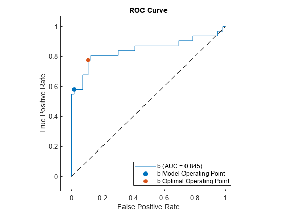
Display the model operating point and the optimal operating point.
modelpt(3,:) = table({"b optimal"},optpt(1),optpt(2),optpt(3))modelpt=3×4 table
ClassName Threshold FalsePositiveRate TruePositiveRate
_______________ _________ _________________ ________________
{'b' } 1.2654 0.017857 0.58065
{'g' } 0.21911 0.41935 0.98214
{["b optimal"]} -1.1978 0.10714 0.77419
Classify XTest using the optimal operating point. Assign an observation whose adjusted score is greater than or equal to the optimal threshold to the positive class b.
s = Scores(:,1) - Scores(:,2);
idx_b_opt = (s >= optpt(1));
Y2 = cell(size(YTest));
Y2(idx_b_opt) = {'b'};
Y2(~idx_b_opt) = {'g'};
Display the adjusted scores for the observations that have different labels in Y1 (labels from the predict function) and Y2 (labels from the optimal threshold optpt(1)).
s(~strcmp(Y1,Y2))
ans = 11×1

   -1.1703
   -0.8445
   -0.8235
   -0.4546
   -1.0719
   -0.4612
   -0.2191
   -1.1978
   -1.0114
   -1.1552
   -0.4525
Eleven observations have adjusted scores less than 0 but greater than or equal to the optimal threshold.
After training a model for a multiclass classification problem, create a rocmetrics object for classes of interest only. Specify FixedMetricValues so that rocmetrics computes the performance metrics for the specified threshold values.
Read the sample file CreditRating_Historical.dat into a table. The predictor data consists of financial ratios and industry sector information for a list of corporate customers. The response variable consists of credit ratings assigned by a rating agency. Preview the first few rows of the data set.
creditrating = readtable("CreditRating_Historical.dat");
head(creditrating)
ID WC_TA RE_TA EBIT_TA MVE_BVTD S_TA Industry Rating
_____ ______ ______ _______ ________ _____ ________ _______
62394 0.013 0.104 0.036 0.447 0.142 3 {'BB' }
48608 0.232 0.335 0.062 1.969 0.281 8 {'A' }
42444 0.311 0.367 0.074 1.935 0.366 1 {'A' }
48631 0.194 0.263 0.062 1.017 0.228 4 {'BBB'}
43768 0.121 0.413 0.057 3.647 0.466 12 {'AAA'}
39255 -0.117 -0.799 0.01 0.179 0.082 4 {'CCC'}
62236 0.087 0.158 0.049 0.816 0.324 2 {'BBB'}
39354 0.005 0.181 0.034 2.597 0.388 7 {'AA' }
Because each value in the ID variable is a unique customer ID, that is, length(unique(creditrating.ID)) is equal to the number of observations in creditrating, the ID variable is a poor predictor. Remove the ID variable from the table, and convert the Industry variable to a categorical variable.
creditrating = removevars(creditrating,"ID");
creditrating.Industry = categorical(creditrating.Industry);
Partition the data into training and test sets. Use approximately 80% of the observations to train a neural network model, and 20% of the observations to test the performance of the trained model on new data. Partition the data using cvpartition.
rng("default") % For reproducibility of the partition
c = cvpartition(creditrating.Rating,"Holdout",0.20);
trainingIndices = training(c); % Indices for the training set
testIndices = test(c); % Indices for the test set
creditTrain = creditrating(trainingIndices,:);
creditTest = creditrating(testIndices,:);
Train a neural network classifier by passing the training data creditTrain to the fitcnet function.
Mdl = fitcnet(creditTrain,"Rating");Compute classification scores and predict credit ratings for the test set observations.
[labels,Scores] = predict(Mdl,creditTest);
The classification scores for a neural network classifier correspond to posterior probabilities.
Assume that you want to evaluate the model only for the ratings B, BB, and BBB, and ignore the rest of the ratings.
Display the order of the ratings in the model stored in the ClassNames property, and identify the classes to evaluate.
Mdl.ClassNames
ans = 7×1 cell
    {'A'  }
    {'AA' }
    {'AAA'}
    {'B'  }
    {'BB' }
    {'BBB'}
    {'CCC'}
idx_Class = [4 5 6];
classesToEvaluate = Mdl.ClassNames(idx_Class);
Find the indices of the observations for the three classes (B, BB, BBB).
idx = ismember(creditTest.Rating,classesToEvaluate);
Create a rocmetrics object using the true labels and scores for the three classes. Specify FixedMetricValues=1:-0.25:-1 so that rocmetrics computes the performance metrics for the specified threshold values.
thresholds = 1:-0.25:-1;
rocObj = rocmetrics(creditTest.Rating(idx),Scores(idx,idx_Class), ...
    classesToEvaluate,FixedMetricValues=thresholds);
Display the computed metrics stored in the Metrics property.
rocObj.Metrics
ans=27×4 table
    ClassName    Threshold    FalsePositiveRate    TruePositiveRate
    _________    _________    _________________    ________________

     {'B' }         0.9165               0                   0
     {'B' }        0.78252               0             0.10938
     {'B' }        0.50068        0.007732             0.32812
     {'B' }        0.28913        0.020619             0.42188
     {'B' }      0.0087441        0.046392             0.57812
     {'B' }       -0.24191         0.10567              0.6875
     {'B' }       -0.48432         0.16753                0.75
     {'B' }       -0.74983         0.51546               0.875
     {'B' }       -0.97077               1                   1
     {'BB'}        0.95598               0                   0
     {'BB'}        0.75365        0.041199             0.18919
     {'BB'}        0.50119         0.10861             0.45946
     {'BB'}        0.25592         0.14981             0.61622
     {'BB'}      0.0044979         0.23221             0.75676
     {'BB'}       -0.23726         0.33708             0.85946
     {'BB'}       -0.49788         0.47191             0.93514
      ⋮
The Metrics property contains the performance metrics for the three ratings B, BB, and BBB and the specified threshold values only. The default UseNearestNeighbor value is true if rocmetrics does not compute confidence intervals. Therefore, for each specified threshold value, rocmetrics selects an adjusted score value nearest to the specified value and uses the nearest value as a threshold. Display the specified threshold values and the actual threshold values used for each class.
idx_B = strcmp(rocObj.Metrics.ClassName,"B");
idx_BB = strcmp(rocObj.Metrics.ClassName,"BB");
idx_BBB = strcmp(rocObj.Metrics.ClassName,"BBB");
table(thresholds',rocObj.Metrics.Threshold(idx_B), ...
    rocObj.Metrics.Threshold(idx_BB), ...
    rocObj.Metrics.Threshold(idx_BBB), ...
    VariableNames=["Fixed Threshold";string(classesToEvaluate)])
ans=9×4 table
    Fixed Threshold        B           BB          BBB
    _______________    _________    _________    ________

             1            0.9165      0.95598     0.93657
          0.75           0.78252      0.75365     0.75513
           0.5           0.50068      0.50119     0.50095
          0.25           0.28913      0.25592     0.25203
             0         0.0087441    0.0044979    0.026637
         -0.25          -0.24191     -0.23726    -0.23003
          -0.5          -0.48432     -0.49788     -0.4998
         -0.75          -0.74983     -0.74749     -0.7479
            -1          -0.97077     -0.93657    -0.96407