3 次元シミュレーション データを使用した深層学習セマンティック セグメンテーション ネットワークの学習

この例では、3 次元シミュレーション データを使用してセマンティック セグメンテーション ネットワークに学習させ、敵対的生成ネットワーク (GAN) を使用して現実のデータに合わせて微調整する方法を示します。

この例では、ドライビング シナリオ デザイナーと Unreal Engine® によって生成された 3 次元シミュレーション データを使用します。このようなシミュレーション データを生成する方法を示す例については、Depth and Semantic Segmentation Visualization Using Unreal Engine Simulation (Automated Driving Toolbox)を参照してください。3 次元シミュレーション環境は、イメージおよび対応するグラウンド トゥルース ピクセル ラベルを生成します。シミュレーション データを使用すると、手間がかかり多大の労力を要する注釈プロセスを回避できます。しかし、シミュレーション データのみで学習された領域シフト モデルは、現実のデータ セットでうまく機能しません。これに対処するには、領域適応を使用して学習済みモデルを微調整し、現実のデータ セットで機能するようにします。

この例では AdaptSegNet [1] を使用します。これは、入力領域に関係なく同じように見える出力セグメンテーション予測の構造を適応させるネットワークです。AdaptSegNet ネットワークは GAN モデルに基づいており、両方のパフォーマンスを最大化するために同時に学習される次の 2 つのネットワークで構成されます。

1. ジェネレーター — 実際の入力イメージまたはシミュレートされた入力イメージから高品質のセグメンテーション結果を生成するように学習されたネットワーク

2. ディスクリミネーター — ジェネレーターのセグメンテーション予測が実データからのものかシミュレートされたデータからのものかを比較して識別を試みるネットワーク

AdaptSegNet モデルを実際のデータに合わせて微調整するために、この例では CamVid データ [2] のサブセットを使用し、モデルを適応させて、CamVid データで高品質のセグメンテーション予測を生成します。

事前学習済みのネットワークのダウンロード

事前学習済みのネットワークをダウンロードします。事前学習済みのモデルを使用することで、学習の完了を待つことなく例全体を実行することができます。ネットワークに学習させる場合は、変数 doTraining を true に設定します。

doTraining = false;
if ~doTraining
    pretrainedURL = 'https://ssd.mathworks.com/supportfiles/vision/data/trainedAdaptSegGANNet.mat';
    pretrainedFolder = fullfile(tempdir,'pretrainedNetwork');
    pretrainedNetwork = fullfile(pretrainedFolder,'trainedAdaptSegGANNet.mat'); 
    if ~exist(pretrainedNetwork,'file')
        mkdir(pretrainedFolder);
        disp('Downloading pretrained network (57 MB)...');
        websave(pretrainedNetwork,pretrainedURL);
    end
    pretrained = load(pretrainedNetwork);
end    

データ セットのダウンロード

この例の「サポート関数」の節で定義されている関数 downloadDataset を使用して、シミュレーション データ セットと実データ セットをダウンロードします。関数 downloadDataset は、CamVid データ セット全体をダウンロードし、データを学習セットとテスト セットに分割します。

シミュレーション データ セットは、ドライビング シナリオ デザイナーによって生成されました。生成されたシナリオは、ラベル付きの 553 のフォトリアリスティックなイメージで構成され、Unreal Engine によってレンダリングされました。このデータ セットを使用して、モデルに学習させます。

実データ セットは、Cambridge University の CamVid データ セットのサブセットです。モデルを現実のデータに適合させるために、69 の CamVid イメージを使用します。学習済みモデルを評価するために、368 の CamVid イメージを使用します。

ダウンロード時間はお使いのインターネット接続によって異なります。

simulationDataURL = 'https://ssd.mathworks.com/supportfiles/vision/data/SimulationDrivingDataset.zip';
realImageDataURL = 'http://web4.cs.ucl.ac.uk/staff/g.brostow/MotionSegRecData/files/701_StillsRaw_full.zip';
realLabelDataURL = 'http://web4.cs.ucl.ac.uk/staff/g.brostow/MotionSegRecData/data/LabeledApproved_full.zip';

simulationDataLocation = fullfile(tempdir,'SimulationData');
realDataLocation = fullfile(tempdir,'RealData');
[simulationImagesFolder, simulationLabelsFolder, realImagesFolder, realLabelsFolder, ...
    realTestImagesFolder, realTestLabelsFolder] = ... 
    downloadDataset(simulationDataLocation,simulationDataURL,realDataLocation,realImageDataURL,realLabelDataURL);

ダウンロードされたファイルには、実領域のピクセル ラベルが含まれていますが、学習プロセスではこれらのピクセル ラベルを使用しないことに注意してください。この例では、実領域のピクセル ラベルのみを使用して、平均の Intersection over Union (IoU) 値を計算し、学習済みモデルの有効性を評価します。

負荷シミュレーションと実データ

imageDatastoreを使用して、学習用のシミュレーション データ セットと実データ セットを読み込みます。イメージ データストアを使用すると、ディスク上の大規模なイメージ コレクションを効率的に読み込むことができます。

simData = imageDatastore(simulationImagesFolder);
realData = imageDatastore(realImagesFolder);

シミュレーション データ セットと実データ セットからイメージをプレビューします。

simImage = preview(simData);
realImage = preview(realData);
montage({simImage,realImage})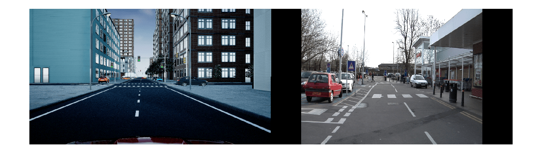

実イメージとシミュレートされたイメージは大きく異なります。結果として、シミュレートされたデータで学習され実データで評価されたモデルは、領域シフトのためにうまく機能しません。

シミュレーション データと実データのピクセル ラベル付きイメージの読み込み

pixelLabelDatastore (Computer Vision Toolbox)を使用してシミュレーション ピクセル ラベル イメージ データを読み込みます。ピクセル ラベル データストアは、ピクセル ラベル データとラベル ID をクラス名マッピングにカプセル化します。

この例では、自動運転アプリケーションに役立つ 5 つのクラス (道路、背景、歩道、空、自動車) を指定します。

classes = [
    "Road"
    "Background"
    "Pavement"
    "Sky"
    "Car"
    ];
numClasses = numel(classes);

シミュレーション データ セットには 8 つのクラスがあります。元のデータ セットの建物、樹木、信号機、照明のクラスを 1 つの背景クラスにグループ化して、クラスの数を 8 から 5 に減らします。補助関数 simulationPixelLabelIDs を使用して、グループ化されたラベル ID を返します。この補助関数は、この例にサポート ファイルとして添付されています。

labelIDs = simulationPixelLabelIDs;

クラスとラベル ID を使用して、シミュレーション データのピクセル ラベル データストアを作成します。

simLabels = pixelLabelDatastore(simulationLabelsFolder,classes,labelIDs);

「サポート関数」の節で定義されている補助関数 domainAdaptationColorMap を使用して、セグメント化されたイメージのカラーマップを初期化します。

dmap = domainAdaptationColorMap;

関数labeloverlay (Image Processing Toolbox)を使用し、イメージの上にラベルを重ね合わせて、ピクセル ラベルの付いたイメージをプレビューします。

simImageLabel = preview(simLabels);
overlayImageSimulation = labeloverlay(simImage,simImageLabel,'ColorMap',dmap);
figure
imshow(overlayImageSimulation)
labelColorbar(dmap,classes);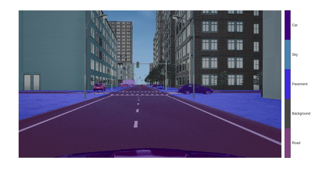

関数transformと「サポート関数」の節で定義されている補助関数 preprocessData を使用し、学習に使用されるシミュレーション データと実データをゼロ中心にシフトして、データを原点の中心に配置します。

preprocessedSimData = transform(simData, @(simdata)preprocessData(simdata));
preprocessedRealData = transform(realData, @(realdata)preprocessData(realdata));

関数combineを使用して、変換後のイメージ データストアとシミュレーション領域のピクセル ラベル データストアを結合します。学習プロセスでは、実データのピクセル ラベルは使用されません。

combinedSimData = combine(preprocessedSimData,simLabels);

AdaptSegNet ジェネレーターの定義

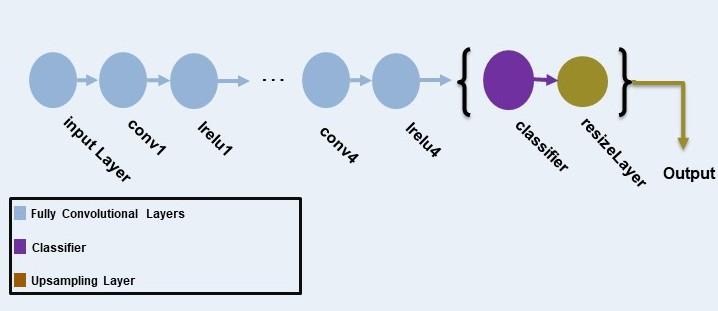
この例では、ImageNet で事前学習済みの VGG-16 ネットワークを完全畳み込みネットワークに変更します。受容野を拡大するために、ストライドが 2 と 4 の拡張畳み込み層を追加します。これにより、出力特徴マップの解像度が入力サイズの 8 分の 1 になります。Atrous Spatial Pyramid Pooling (ASPP) を使用してマルチスケール情報を提供した後、アップサンプリング係数を 8 とする resize2dlayer を使用して出力のサイズを入力のサイズに変更します。

この例で使用する AdaptSegNet ジェネレーター ネットワークを次の図に示します。

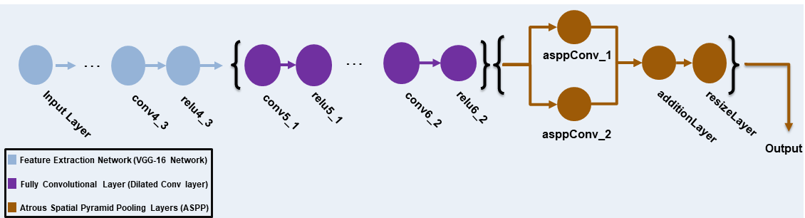
事前学習済みの VGG-16 ネットワークを取得するには、vgg16をインストールします。サポート パッケージがインストールされていない場合、ダウンロード用リンクが表示されます。

[net,~] = imagePretrainedNetwork('vgg16'); 

VGG-16 ネットワークをセマンティック セグメンテーションに適したものにするには、'relu4_3' の後のすべての VGG 層を削除します。

vggLayers = net.Layers(2:24);

ジェネレーター用に 1280 x 720 x 3 のサイズのイメージ入力層を作成します。

inputSizeGenerator = [1280 720 3];
inputLayer = imageInputLayer(inputSizeGenerator,'Normalization','None','Name','inputLayer');

完全畳み込みネットワーク層を作成します。膨張係数に 2 と 4 を使用して、それぞれのフィールドを拡大します。

fcnlayers = [
    convolution2dLayer([3 3], 360,'DilationFactor',[2 2],'Padding',[2 2 2 2],'Name','conv5_1','WeightsInitializer','narrow-normal','BiasInitializer','zeros')
    reluLayer('Name','relu5_1')
    convolution2dLayer([3 3], 360,'DilationFactor',[2 2],'Padding',[2 2 2 2] ,'Name','conv5_2','WeightsInitializer','narrow-normal','BiasInitializer','zeros')
    reluLayer('Name','relu5_2')
    convolution2dLayer([3 3], 360,'DilationFactor',[2 2],'Padding',[2 2 2 2],'Name','conv5_3','WeightsInitializer','narrow-normal','BiasInitializer','zeros')
    reluLayer('Name','relu5_3')
    convolution2dLayer([3 3], 480,'DilationFactor',[4 4],'Padding',[4 4 4 4],'Name','conv6_1','WeightsInitializer','narrow-normal','BiasInitializer','zeros')
    reluLayer('Name','relu6_1')
    convolution2dLayer([3 3], 480,'DilationFactor',[4 4],'Padding',[4 4 4 4] ,'Name','conv6_2','WeightsInitializer','narrow-normal','BiasInitializer','zeros')
    reluLayer('Name','relu6_2')
    ];

層を組み合わせてジェネレーター ネットワークを作成します。

layers = [
    inputLayer
    vggLayers
    fcnlayers
    ];
dlnetGenerator = dlnetwork(layers);

ASPP を使用してマルチスケール情報を提供します。「サポート関数」のセクションで定義されている補助関数 addASPPToNetwork を使用して、チャネル数に等しいフィルター サイズで ASPP モジュールをジェネレーター ネットワークに追加します。

dlnetGenerator  = addASPPToNetwork(dlnetGenerator, numClasses);

アップサンプリング係数を 8 として resize2dLayer を適用し、出力を入力のサイズと一致させます。

upSampleLayer = resize2dLayer('Scale',8,'Method','bilinear','Name','resizeLayer');
dlnetGenerator = addLayers(dlnetGenerator,upSampleLayer);
dlnetGenerator = connectLayers(dlnetGenerator,'additionLayer','resizeLayer');

ジェネレーター ネットワークをプロットで可視化します。

plot(dlnetGenerator)
title("Generator")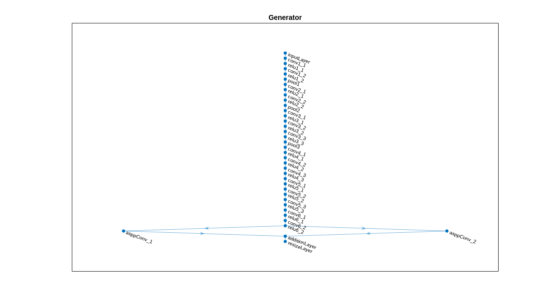

AdaptSeg ディスクリミネーターの定義

ディスクリミネーター ネットワークは、カーネル サイズ 3、ストライド 2 の 5 つの畳み込み層で構成されます。チャネル数は {64, 128, 256, 512, 1} です。最後の層を除いて、各層の後には、0.2 のスケールでパラメーター化された leaky ReLU 層が続きます。resize2dLayer を使用して、ディスクリミネーターの出力のサイズを変更します。この例ではバッチ正規化を使用しないことに注意してください。これは、小さなバッチ サイズを使用してディスクリミネーターをセグメンテーション ネットワークと共同で学習させるためです。

この例の AdaptSegNet ディスクリミネーター ネットワークを次の図に示します。

シミュレーション領域と実領域のセグメンテーション予測を取り込む、1280 x 720 x numClasses のサイズのイメージ入力層を作成します。

inputSizeDiscriminator = [1280 720 numClasses];

完全畳み込み層を作成し、ディスクリミネーター ネットワークを生成します。

% Factor for number of channels in convolution layer.
numChannelsFactor = 64;

% Scale factor to resize the output of the discriminator.
resizeScale = 64;

% Scalar multiplier for leaky ReLU layers.
leakyReLUScale = 0.2;

% Create the layers of the discriminator.
layers = [
    imageInputLayer(inputSizeDiscriminator,'Normalization','none','Name','inputLayer')
    convolution2dLayer(3,numChannelsFactor,'Stride',2,'Padding',1,'Name','conv1','WeightsInitializer','narrow-normal','BiasInitializer','narrow-normal')
    leakyReluLayer(leakyReLUScale,'Name','lrelu1')
    convolution2dLayer(3,numChannelsFactor*2,'Stride',2,'Padding',1,'Name','conv2','WeightsInitializer','narrow-normal','BiasInitializer','narrow-normal')
    leakyReluLayer(leakyReLUScale,'Name','lrelu2')
    convolution2dLayer(3,numChannelsFactor*4,'Stride',2,'Padding',1,'Name','conv3','WeightsInitializer','narrow-normal','BiasInitializer','narrow-normal')
    leakyReluLayer(leakyReLUScale,'Name','lrelu3')
    convolution2dLayer(3,numChannelsFactor*8,'Stride',2,'Padding',1,'Name','conv4','WeightsInitializer','narrow-normal','BiasInitializer','narrow-normal')
    leakyReluLayer(leakyReLUScale,'Name','lrelu4')
    convolution2dLayer(3,1,'Stride',2,'Padding',1,'Name','classifer','WeightsInitializer','narrow-normal','BiasInitializer','narrow-normal')
    resize2dLayer('Scale', resizeScale,'Method','bilinear','Name','resizeLayer');
    ];

% Create the dlnetwork of the discriminator.
dlnetDiscriminator  = dlnetwork(layers);

ディスクリミネーター ネットワークをプロットで可視化します。

plot(dlnetDiscriminator)
title("Discriminator")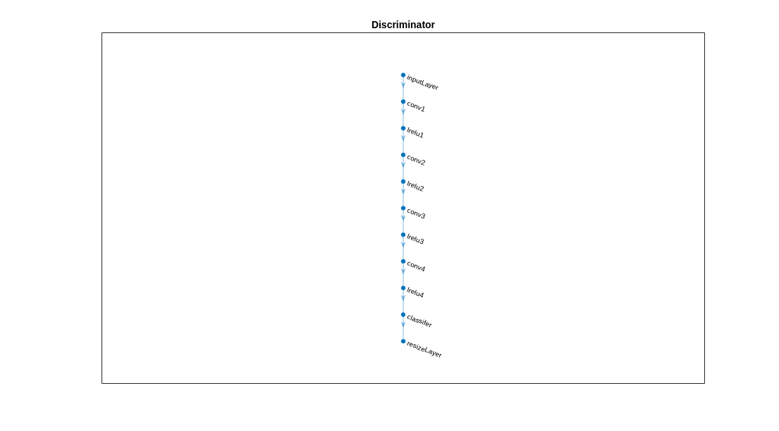

学習オプションの指定

これらの学習オプションを指定します。

• 反復の総数を 5000 に設定。これにより、ネットワークの学習を約 10 エポック行います。

• ジェネレーターの学習率を 2.5e-4 に設定。

• ディスクリミネーターの学習率を 1e-4 に設定。

• L2 正則化係数を 0.0005 に設定。

• 学習率を式 $$learningrate\times$$ $$[\frac{iteration}{totaliterations}{]}^{power}$$ に基づいて指数関数的に減少。このように減少することで、より高い反復数で勾配が安定するようになります。power を 0.9 に設定。

• 敵対的損失の重みを 0.001 に設定。

• 勾配の速度を [ ] として初期化。この値は、勾配の速度を格納するために SGDM によって使用されます。

• パラメーター勾配の移動平均を [ ] として初期化。この値は、パラメーター勾配の平均を格納するために Adam 初期化子によって使用されます。

• 二乗パラメーター勾配の移動平均を [ ] として初期化。この値は、二乗パラメーター勾配の平均を格納するために Adam 初期化子によって使用されます。

• ミニバッチのサイズを 1 に設定。

numIterations = 5000;
learnRateGenBase = 2.5e-4;
learnRateDisBase = 1e-4;
l2Regularization = 0.0005;
power = 0.9;
lamdaAdv = 0.001;
vel= [];
averageGrad = [];
averageSqGrad = [];
miniBatchSize = 1;

GPU が利用できる場合、GPU で学習を行います。GPU を使用するには、Parallel Computing Toolbox™、および CUDA® 対応の NVIDIA® GPU が必要です。使用できる GPU が存在するか自動的に検出するには、executionEnvironment を "auto" に設定します。GPU がない場合、または学習で GPU を使用しない場合は、executionEnvironment を "cpu" に設定します。学習に GPU が使用されるようにするために、executionEnvironment を "gpu" に設定します。サポートされる Compute Capability の詳細については、GPU 計算の要件 (Parallel Computing Toolbox)を参照してください。

executionEnvironment = "auto";

シミュレーション領域の結合されたデータストアからminibatchqueueオブジェクトを作成します。

mbqTrainingDataSimulation =  minibatchqueue(combinedSimData,"MiniBatchSize",miniBatchSize, ...
    "MiniBatchFormat","SSCB","OutputEnvironment",executionEnvironment);

実領域の入力イメージ データストアからminibatchqueueオブジェクトを作成します。

mbqTrainingDataReal = minibatchqueue(preprocessedRealData,"MiniBatchSize",miniBatchSize, ... 
    "MiniBatchFormat","SSCB","OutputEnvironment",executionEnvironment);

モデルの学習

カスタム学習ループを使用してモデルに学習させます。この例の「サポート関数」の節で定義されている補助関数 modelGradients は、ジェネレーターとディスクリミネーターの勾配と損失を計算します。この例にサポート ファイルとして添付されている configureTrainingLossPlotter を使用して学習の進行状況プロットを作成し、updateTrainingPlots を使用して学習の進行状況を更新します。学習データ全体をループ処理し、各反復でネットワーク パラメーターを更新します。

それぞれの反復で次を行います。

• 関数nextを使用して、シミュレーション データの minibatchqueue オブジェクトからイメージとラベルの情報を読み取る。

• 関数nextを使用して、実データの minibatchqueue オブジェクトからイメージ情報を読み取る。

• dlfevalと、「サポート関数」の節で定義されている補助関数 modelGradients を使用してモデルの勾配を評価。modelGradients は、学習可能なパラメーターに関する損失の勾配を返します。

• 関数sgdmupdateを使用してジェネレーターのネットワーク パラメーターを更新。

• 関数adamupdateを使用してディスクリミネーターのネットワーク パラメーターを更新。

• 反復のたびに学習の進行状況プロットを更新し、計算されたさまざまな損失を表示します。

if doTraining

    % Initialize the dlnetwork object of the generator.
    dlnetGenerator = initialize(dlnetGenerator);
    
    % Initialize the dlnetwork object of the discriminator.
    dlnetDiscriminator = initialize(dlnetDiscriminator);
    
    % Create the subplots for the generator and discriminator loss.
    fig = figure;
    [generatorLossPlotter, discriminatorLossPlotter] = configureTrainingLossPlotter(fig);
    
    % Loop through the data for the specified number of iterations.
    for iter = 1:numIterations
       
        % Reset the minibatchqueue of simulation data.
        if ~hasdata(mbqTrainingDataSimulation)
            reset(mbqTrainingDataSimulation);
        end
        
        % Retrieve the next mini-batch of simulation data and labels.
        [dlX,label] = next(mbqTrainingDataSimulation); 
        
        % Reset the minibatchqueue of real data.
        if ~hasdata(mbqTrainingDataReal)
            reset(mbqTrainingDataReal);
        end
        
        % Retrieve the next mini-batch of real data. 
        dlZ = next(mbqTrainingDataReal);  
        
        % Evaluate the model gradients and loss using dlfeval and the modelGradients function.
        [gradientGenerator,gradientDiscriminator, lossSegValue, lossAdvValue, lossDisValue] = ...
            dlfeval(@modelGradients,dlnetGenerator,dlnetDiscriminator,dlX,dlZ,label,lamdaAdv);
        
        % Apply L2 regularization.
        gradientGenerator  = dlupdate(@(g,w) g + l2Regularization*w, gradientGenerator, dlnetGenerator.Learnables);
        
        % Adjust the learning rate.
        learnRateGen = piecewiseLearningRate(iter,learnRateGenBase,numIterations,power);
        learnRateDis = piecewiseLearningRate(iter,learnRateDisBase,numIterations,power);
        
         % Update the generator network learnable parameters using the SGDM optimizer.
        [dlnetGenerator.Learnables, vel] = ... 
            sgdmupdate(dlnetGenerator.Learnables,gradientGenerator,vel,learnRateGen);
               
         % Update the discriminator network learnable parameters using the Adam optimizer.
        [dlnetDiscriminator.Learnables, averageGrad, averageSqGrad] = ...
            adamupdate(dlnetDiscriminator.Learnables,gradientDiscriminator,averageGrad,averageSqGrad,iter,learnRateDis) ;
        
        % Update the training plot with loss values.
        updateTrainingPlots(generatorLossPlotter,discriminatorLossPlotter,iter, ... 
            double(gather(extractdata(lossSegValue + lamdaAdv * lossAdvValue))),double(gather(extractdata(lossDisValue))));

    end
    
    % Save the trained model.
    save('trainedAdaptSegGANNet.mat','dlnetGenerator');
else
    % Load the pretrained generator model to dlnetGenerator.
    dlnetGenerator = pretrained.dlnetGenerator;
end

ディスクリミネーターが、入力がシミュレーションからのものか、実領域からのものかを識別できるようになりました。他方、ジェネレーターは、シミュレーション領域と実領域で類似するセグメンテーション予測を生成できるようになりました。

実際のテスト データでのモデルの評価

テスト データ予測の平均 IoU を計算することにより、学習済みの AdaptSegNet ネットワークのパフォーマンスを評価します。

imageDatastoreを使用してテスト データを読み込みます。

realTestData = imageDatastore(realTestImagesFolder);

CamVid データ セットには 32 のクラスがあります。シミュレーション データ セットの場合と同様に、補助関数 realpixelLabelIDs を使用してクラスの数を 5 つに減らします。補助関数 realpixelLabelIDs は、この例にサポート ファイルとして添付されています。

labelIDs = realPixelLabelIDs;

pixelLabelDatastore (Computer Vision Toolbox)を使用して、テスト データのグラウンド トゥルース ラベル イメージを読み込みます。

realTestLabels = pixelLabelDatastore(realTestLabelsFolder,classes,labelIDs);

関数transformと、「サポート関数」の節で定義されている補助関数 preprocessData を使用して、学習データと同様に、ゼロ中心にデータをシフトして原点を中心にデータを配置します。

preprocessedRealTestData = transform(realTestData, @(realtestdata)preprocessData(realtestdata));

combineを使用して、変換後のイメージ データストアと実際のテスト データのピクセル ラベル データストアを結合します。

combinedRealTestData = combine(preprocessedRealTestData,realTestLabels);

テスト データの結合されたデータストアからminibatchqueueオブジェクトを作成します。. メトリクスの評価を容易にするために、"MiniBatchSize" を 1 に設定します。

mbqimdsTest = minibatchqueue(combinedRealTestData,"MiniBatchSize",1,...
    "MiniBatchFormat","SSCB","OutputEnvironment",executionEnvironment);

混同行列 cell 配列を生成するには、テスト データの minibatchqueue オブジェクトで補助関数 predictSegmentationLabelsOnTestSet を使用します。補助関数 predictSegmentationLabelsOnTestSet は、以下の「サポート関数」の節にリストされています。

imageSetConfusionMat = predictSegmentationLabelsOnTestSet(dlnetGenerator,mbqimdsTest);

evaluateSemanticSegmentation (Computer Vision Toolbox)を使用して、テスト セット混同行列のセマンティック セグメンテーション メトリクスを測定します。

metrics = evaluateSemanticSegmentation(imageSetConfusionMat,classes,'Verbose',false);

データ セット レベルのメトリクスを確認するには、metrics.DataSetMetrics を検査します。

metrics.DataSetMetrics

ans=1×4 table
    GlobalAccuracy    MeanAccuracy    MeanIoU    WeightedIoU
    ______________    ____________    _______    ___________

       0.86883          0.76899       0.64487      0.78026  

データ セット メトリクスは、ネットワーク パフォーマンスの概要を提供します。各クラスがパフォーマンス全体に与える影響を確認するには、metrics.ClassMetrics を使用してクラスごとのメトリクスを検査します。

metrics.ClassMetrics

ans=5×2 table
                  Accuracy      IoU  
                  ________    _______

    Road          0.91471     0.81302
    Background     0.9342     0.85518
    Pavement      0.33376     0.27107
    Sky           0.82647     0.81105
    Car           0.83581     0.47404

データ セットのパフォーマンスは良好ですが、クラス メトリクスは、自動車と歩道のクラスが適切にセグメント化されていないことを示しています。追加のデータを使用してネットワークに学習させることで、結果を改善できます。

イメージのセグメント化

学習済みのネットワークを 1 つのテスト イメージで実行して、セグメント化された出力予測をチェックします。

% Read the image from the test data.
data = readimage(realTestData,350);

% Perform the preprocessing step of zero shift on the image.
processeddata = preprocessData(data);

% Convert the data to dlarray.
processeddata = dlarray(processeddata,'SSCB');

% Predict the output of the network.
[genPrediction, ~] = forward(dlnetGenerator,processeddata);

% Get the label, which is the index with the maximum value in the channel dimension.
[~, labels] = max(genPrediction,[],3);

% Overlay the predicted labels on the image.
segmentedImage = labeloverlay(data,uint8(gather(extractdata(labels))),'Colormap',dmap);

結果を表示します。

figure
imshow(segmentedImage);
labelColorbar(dmap,classes);

ラベルの結果を、realTestLabels に格納されているグラウンド トゥルースの予想と比較します。緑とマゼンタの領域は、セグメンテーション結果が予想されるグラウンド トゥルースと異なる領域を強調表示しています。

expectedResult = readimage(realTestLabels,350);
actual = uint8(gather(extractdata(labels)));
expected = uint8(expectedResult);
figure
imshowpair(actual,expected)

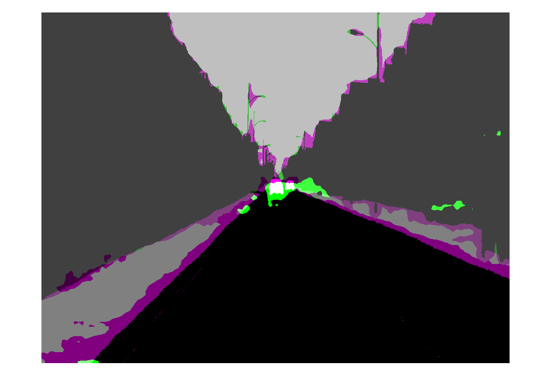
視覚的には、道路、空、建物などのクラスでセマンティック セグメンテーションの結果が適切にオーバーラップしています。ただし、車と歩道のクラスでは結果が適切にオーバーラップしていません。

サポート関数

モデル勾配関数

補助関数 modelGradients は、ジェネレーターとディスクリミネーターの勾配と敵対的損失を計算します。この関数は、ジェネレーターのセグメンテーション損失とディスクリミネーターのクロスエントロピー損失も計算します。ジェネレーター ネットワークとディスクリミネーター ネットワークの両方の反復間で状態情報を保持する必要がないため、状態は更新されません。

function [gradientGenerator, gradientDiscriminator, lossSegValue, lossAdvValue, lossDisValue] = modelGradients(dlnetGenerator, dlnetDiscriminator, dlX, dlZ, label, lamdaAdv)

% Labels for adversarial training.
simulationLabel = 0;
realLabel = 1;

% Extract the predictions of the simulation from the generator.
[genPredictionSimulation, ~] = forward(dlnetGenerator,dlX);

% Compute the generator loss.
lossSegValue = segmentationLoss(genPredictionSimulation,label);

% Extract the predictions of the real data from the generator.
[genPredictionReal, ~] = forward(dlnetGenerator,dlZ);

% Extract the softmax predictions of the real data from the discriminator.
disPredictionReal = forward(dlnetDiscriminator,softmax(genPredictionReal));

% Create a matrix of simulation labels of real prediction size.
Y = simulationLabel * ones(size(disPredictionReal));

% Compute the adversarial loss to make the real distribution close to the simulation label.
lossAdvValue = mse(disPredictionReal,Y)/numel(Y(:));

% Compute the gradients of the generator with regard to loss.
gradientGenerator = dlgradient(lossSegValue + lamdaAdv*lossAdvValue,dlnetGenerator.Learnables);

% Extract the softmax predictions of the simulation from the discriminator.
disPredictionSimulation = forward(dlnetDiscriminator,softmax(genPredictionSimulation));

% Create a matrix of simulation labels of simulation prediction size.
Y = simulationLabel * ones(size(disPredictionSimulation));

% Compute the discriminator loss with regard to simulation class.
lossDisValueSimulation = mse(disPredictionSimulation,Y)/numel(Y(:));
 
% Extract the softmax predictions of the real data from the discriminator.
disPredictionReal = forward(dlnetDiscriminator,softmax(genPredictionReal));

% Create a matrix of real labels of real prediction size.
Y = realLabel * ones(size(disPredictionReal));

% Compute the discriminator loss with regard to real class.
lossDisValueReal = mse(disPredictionReal,Y)/numel(Y(:));

% Compute the total discriminator loss.
lossDisValue = lossDisValueSimulation + lossDisValueReal;

% Compute the gradients of the discriminator with regard to loss.
gradientDiscriminator = dlgradient(lossDisValue,dlnetDiscriminator.Learnables);

end

損失関数のセグメンテーション

補助関数 segmentationLoss は、シミュレーション データとそれぞれのグラウンド トゥルースを使用して、ジェネレーターのクロスエントロピー損失として定義される特徴セグメンテーション損失を計算します。補助関数は、関数crossentropyを使用して損失を計算します。

function loss = segmentationLoss(predict, target)

% Generate the one-hot encodings of the ground truth.
oneHotTarget = onehotencode(categorical(extractdata(target)),3);

% Convert the one-hot encoded data to dlarray.
oneHotTarget = dlarray(oneHotTarget,'SSCB');

% Compute the softmax output of the predictions.
predictSoftmax = softmax(predict);

% Mask to ignore nans.
mask = ~isnan(oneHotTarget);

% Compute the cross-entropy loss.
loss =  crossentropy(predictSoftmax,oneHotTarget,'ClassificationMode','single-label','Mask',mask)/(numel(oneHotTarget)/2);
end

補助関数 downloadDataset は、シミュレーション データ セットと実データ セットの両方が存在しない場合に、指定された URL から、指定されたフォルダーの場所にそれらをダウンロードします。この関数は、シミュレーションのパス、実際の学習データ、および実際のテスト データを返します。この関数は、CamVid データ セット全体をダウンロードし、この例にサポート ファイルとして添付されている subsetCamVidDatasetFileNames.mat ファイルを使用して、データを学習セットとテスト セットに分割します。

function [simulationImagesFolder, simulationLabelsFolder, realImagesFolder, realLabelsFolder,...
    realTestImagesFolder, realTestLabelsFolder] = ...
    downloadDataset(simulationDataLocation, simulationDataURL, realDataLocation, realImageDataURL, realLabelDataURL)
    
% Build the training image and label folder location for simulation data.
simulationDataZip = fullfile(simulationDataLocation,'SimulationDrivingDataset.zip');

% Get the simulation data if it does not exist.
if ~exist(simulationDataZip,'file')
    mkdir(simulationDataLocation)
    
    disp('Downloading the simulation data');
    websave(simulationDataZip,simulationDataURL);
    unzip(simulationDataZip,simulationDataLocation);
end
  
simulationImagesFolder = fullfile(simulationDataLocation,'SimulationDrivingDataset','images');
simulationLabelsFolder = fullfile(simulationDataLocation,'SimulationDrivingDataset','labels');

camVidLabelsZip = fullfile(realDataLocation,'CamVidLabels.zip');
camVidImagesZip = fullfile(realDataLocation,'CamVidImages.zip');

if ~exist(camVidLabelsZip,'file') || ~exist(camVidImagesZip,'file')   
    mkdir(realDataLocation)
       
    disp('Downloading 16 MB CamVid dataset labels...'); 
    websave(camVidLabelsZip, realLabelDataURL);
    unzip(camVidLabelsZip, fullfile(realDataLocation,'CamVidLabels'));
    
    disp('Downloading 587 MB CamVid dataset images...');  
    websave(camVidImagesZip, realImageDataURL);       
    unzip(camVidImagesZip, fullfile(realDataLocation,'CamVidImages'));    
end

% Build the training image and label folder location for real data.
realImagesFolder = fullfile(realDataLocation,'train','images');
realLabelsFolder = fullfile(realDataLocation,'train','labels');

% Build the testing image and label folder location for real data.
realTestImagesFolder = fullfile(realDataLocation,'test','images');
realTestLabelsFolder = fullfile(realDataLocation,'test','labels');

% Partition the data into training and test sets if they do not exist.
if ~exist(realImagesFolder,'file') || ~exist(realLabelsFolder,'file') || ...
        ~exist(realTestImagesFolder,'file') || ~exist(realTestLabelsFolder,'file')

    
    mkdir(realImagesFolder);
    mkdir(realLabelsFolder);
    mkdir(realTestImagesFolder);
    mkdir(realTestLabelsFolder);
    
    % Load the mat file that has the names for testing and training.
    partitionNames = load('subsetCamVidDatasetFileNames.mat');
    
    % Extract the test images names.
    imageTestNames = partitionNames.imageTestNames;
    
    % Remove the empty cells. 
    imageTestNames = imageTestNames(~cellfun('isempty',imageTestNames));
    
    % Extract the test labels names.
    labelTestNames = partitionNames.labelTestNames;
    
    % Remove the empty cells.
    labelTestNames = labelTestNames(~cellfun('isempty',labelTestNames));
    
    % Copy the test images to the respective folder.
    for i = 1:size(imageTestNames,1)
        labelSource = fullfile(realDataLocation,'CamVidLabels',labelTestNames(i));
        imageSource = fullfile(realDataLocation,'CamVidImages','701_StillsRaw_full',imageTestNames(i));
        copyfile(imageSource{1}, realTestImagesFolder);
        copyfile(labelSource{1}, realTestLabelsFolder);
    end
    
    % Extract the train images names.
    imageTrainNames = partitionNames.imageTrainNames;
    
    % Remove the empty cells.
    imageTrainNames = imageTrainNames(~cellfun('isempty',imageTrainNames));
    
    % Extract the train labels names.
    labelTrainNames = partitionNames.labelTrainNames;
    
    % Remove the empty cells.
    labelTrainNames = labelTrainNames(~cellfun('isempty',labelTrainNames));
    
    % Copy the train images to the respective folder.
    for i = 1:size(imageTrainNames,1)
        labelSource = fullfile(realDataLocation,'CamVidLabels',labelTrainNames(i));
        imageSource = fullfile(realDataLocation,'CamVidImages','701_StillsRaw_full',imageTrainNames(i));
        copyfile(imageSource{1},realImagesFolder);
        copyfile(labelSource{1},realLabelsFolder);
    end
end
end

補助関数 addASPPToNetwork は、Atrous Spatial Pyramid Pooling (ASPP) 層を作成し、それらを入力 dlnetwork に追加します。この関数は、ASPP 層が接続された dlnetwork を返します。

function net  = addASPPToNetwork(net, numClasses)

% Define the ASPP dilation factors.
asppDilationFactors = [6,12];

% Define the ASPP filter sizes.
asppFilterSizes = [3,3];

% Extract the last layer of the dlnetwork.
lastLayerName = net.Layers(end).Name;

% Define the addition layer.
addLayer = additionLayer(numel(asppDilationFactors),'Name','additionLayer');

% Add the addition layer to the dlnetwork.
net = addLayers(net,addLayer);

% Create the ASPP layers connected to the addition layer
% and connect the dlnetwork.
for i = 1: numel(asppDilationFactors)
    asppConvName = "asppConv_" + string(i);
    branchFilterSize = asppFilterSizes(i);
    branchDilationFactor = asppDilationFactors(i);
    asspLayer  = convolution2dLayer(branchFilterSize, numClasses,'DilationFactor', branchDilationFactor,...
        'Padding','same','Name',asppConvName,'WeightsInitializer','narrow-normal','BiasInitializer','zeros');
    net = addLayers(net,asspLayer);
    net = connectLayers(net,lastLayerName,asppConvName);
    net = connectLayers(net,asppConvName,strcat(addLayer.Name,'/',addLayer.InputNames{i}));
end
end

補助関数 predictSegmentationLabelsOnTestSet は、関数segmentationConfusionMatrix (Computer Vision Toolbox)を使用して予測ラベルとグラウンド トゥルース ラベルの混同行列を計算します。

function confusionMatrix =  predictSegmentationLabelsOnTestSet(net, minbatchTestData)   
    
confusionMatrix = {};
i = 1;
while hasdata(minbatchTestData)
    
    % Use next to retrieve a mini-batch from the datastore.
    [dlX, gtlabels] = next(minbatchTestData);
    
    % Predict the output of the network.
    [genPrediction, ~] = forward(net,dlX);
    
    % Get the label, which is the index with maximum value in the channel dimension.
    [~, labels] = max(genPrediction,[],3);
    
    % Get the confusion matrix of each image.
    confusionMatrix{i}  = segmentationConfusionMatrix(double(gather(extractdata(labels))),double(gather(extractdata(gtlabels))));
  
    i = i+1;
end

confusionMatrix = confusionMatrix';
    
end

補助関数 piecewiseLearningRate は、反復回数に基づいて現在の学習率を計算します。

function lr = piecewiseLearningRate(i, baseLR, numIterations, power)

fraction = i/numIterations;
factor = (1 - fraction)^power * 1e1;
lr = baseLR * factor;

end

補助関数 preprocessData は、イメージ チャネルの数をそれぞれの平均で減算して、ゼロ センター シフトを実行します。

function data = preprocessData(data)

% Extract respective channels.
rc = data(:,:,1);
gc = data(:,:,2);
bc = data(:,:,3);

% Compute the respective channel means.
r = mean(rc(:));
g = mean(gc(:));
b = mean(bc(:));

% Shift the data by the mean of respective channel.
data = single(data) - single(shiftdim([r g b],-1));  
end

参考文献

[1] Tsai, Yi-Hsuan, Wei-Chih Hung, Samuel Schulter, Kihyuk Sohn, Ming-Hsuan Yang, and Manmohan Chandraker. “Learning to Adapt Structured Output Space for Semantic Segmentation.” In 2018 IEEE/CVF Conference on Computer Vision and Pattern Recognition, 7472–81. Salt Lake City, UT: IEEE, 2018. https://doi.org/10.1109/CVPR.2018.00780.

[2] Brostow, Gabriel J., Julien Fauqueur, and Roberto Cipolla.“Semantic Object Classes in Video: A High-Definition Ground Truth Database.” Pattern Recognition Letters 30, no. 2 (January 2009): 88–97. https://doi.org/10.1016/j.patrec.2008.04.005.