Explore Quantized Semantic Segmentation Network Using Grad-CAM
Compare the predictions of a quantized semantic segmentation network to the original network using the gradient-weighted class activation mapping (Grad-CAM) interpretability method.
To run this example, you must have the licenses for the software required to quantize a deep learning network. For information about this software, see Quantization Workflow Prerequisites.
Semantic segmentation involves assigning a class to each pixel in a 2-D image. In this example, you load a network that is trained to perform breast tumor segmentation using the DeepLab v3+ architecture. For more information about how to train this type of network, see Breast Tumor Segmentation from Ultrasound Using Deep Learning. You can then use the Deep Learning Toolbox Model Quantization Library support package to reduce the memory footprint of the network by quantizing the weights, biases, and activations of the convolution layers to 8-bit scaled integer values.
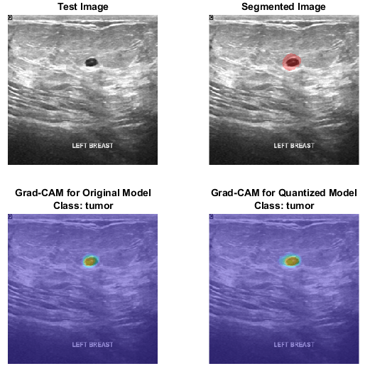
To verify that quantizing of the network does not substantially change its behavior, you can use Grad-CAM, a deep learning interpretability technique. With this technique, you can determine which regions of an image differ in the pixel classification decision between the original, floating-point network and the quantized network.
This figure shows Grad-CAM maps for the original network and the quantized network.
Download Pretrained Network
Download the pretrained DeepLab v3+ network and a test image by using the downloadTrainedNetwork helper function. The helper function is attached to this example as a supporting file. You can use the pretrained network to run the example without training the network. To learn more about how to train this network, see Breast Tumor Segmentation from Ultrasound Using Deep Learning.
dataDir = fullfile(tempdir,"BreastSegmentation");
if ~exist(dataDir,"dir")
    mkdir(dataDir)
end
pretrainedNetwork_url = "https://www.mathworks.com/supportfiles/"+ ...
    "image/data/breastTumorDeepLabV3.tar.gz";
downloadTrainedNetwork(pretrainedNetwork_url,dataDir);
Downloading pretrained network.
This can take several minutes to download...
Done.
Unzip the TAR GZ file. Load the pretrained network.
gunzip(fullfile(dataDir,"breastTumorDeepLabV3.tar.gz"),dataDir);
untar(fullfile(dataDir,"breastTumorDeepLabV3.tar"),dataDir);
exampleDir = fullfile(dataDir,"breastTumorDeepLabV3");
load(fullfile(exampleDir,"breast_seg_deepLabV3.mat"));
Perform Semantic Segmentation
Before you analyze the network predictions, use the pretrained network to segment a test image. Read the test ultrasound image and resize the image to the input size of the pretrained network.
inputSize = trainedNet.Layers(1).InputSize(1:2);

imTest = imread(fullfile(exampleDir,"breastUltrasoundImg.png"));
imTest = imresize(imTest,inputSize);
Predict the tumor segmentation mask for the test image.
segmentedImg = semanticseg(imTest,trainedNet);
Display the test image and the test image with the predicted tumor label overlay as a montage.
overlayImg = labeloverlay(imTest,segmentedImg, ...
    Transparency=0.7, ...
    IncludedLabels="tumor", ...
    Colormap="hsv");
montage({imTest,overlayImg});

Download Data Set
To quantize and test the network, this example uses the Breast Ultrasound Images (BUSI) data set [2]. The BUSI data set contains 2-D ultrasound images in the PNG file format. The total size of the data set is 197 MB. The data set contains 133 normal scans, 487 scans with benign tumors, and 210 scans with malignant tumors. This example uses images from the tumor groups only. Each ultrasound image has a corresponding tumor mask image. The tumor mask labels have been reviewed by clinical radiologists [2].
Run this code to download the dataset from the MathWorks® website and unzip the downloaded folder.
zipFile = matlab.internal.examples.downloadSupportFile("image","data/Dataset_BUSI.zip");
filepath = fileparts(zipFile);
unzip(zipFile,filepath)
The imageDir folder contains the downloaded and unzipped dataset.
imageDir = fullfile(filepath,"Dataset_BUSI_with_GT");Load Data
Import and process the data using the same steps as in the Breast Tumor Segmentation from Ultrasound Using Deep Learning example.
Create an imageDatastore object to read and manage the ultrasound image data. Label each image as normal, benign, or malignant according to the name of its folder.
imds = imageDatastore(imageDir, ...
    IncludeSubfolders=true, ...
    LabelSource="foldernames");
Remove files whose names contain "mask" to remove label images from the datastore. The image datastore now contains only the grayscale ultrasound images.
imds = subset(imds,find(~contains(imds.Files,"mask")));Create a pixelLabelDatastore (Computer Vision Toolbox) object to store the labels.
classNames = ["tumor","background"];
labelIDs = [1 0];
numClasses = numel(classNames);
pxds = pixelLabelDatastore(imageDir,classNames,labelIDs,IncludeSubfolders=true);
Include only the subset of files whose names contain "_mask.png" in the datastore. The pixel label datastore now contains only the tumor mask images.
pxds = subset(pxds,contains(pxds.Files,"_mask.png"));Combine the image datastore and the pixel label datastore to create a CombinedDatastore object.
dsCombined = combine(imds,pxds);
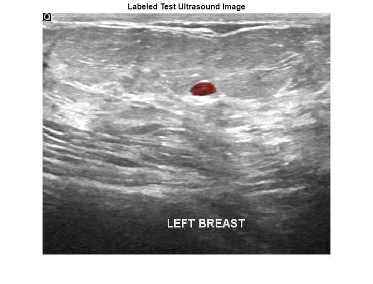
Preview one image with a tumor mask overlay.
testImage  = preview(imds);
mask = preview(pxds);

B = labeloverlay(testImage,mask, ...
    Transparency=0.7, ...
    IncludedLabels="tumor", ...
    Colormap="hsv");
imshow(B)
title("Labeled Test Ultrasound Image")
Prepare Data for Calibration and Validation
Partition Data into Training, Validation, and Test Sets
Split the combined datastore into data sets for training, validation, and testing. Allocate 80% of the data for training, 10% for validation, and the remaining 10% for testing. Determine which indices to include in each set by using the splitlabels (Computer Vision Toolbox) function. To exclude images in the normal class without tumor images, use the image datastore labels as input and set the Exclude name-value argument to "normal".
idxSet = splitlabels(imds.Labels,[0.8 0.1],"randomized",Exclude="normal");
Use the validation data to calibrate the quantized network. Use the test data to assess the performance of the original and quantized networks.
dsVal = subset(dsCombined,idxSet{2});
dsTest = subset(dsCombined,idxSet{3});
Augment Validation Data
Augment the validation data using the transform function with custom preprocessing operations defined in the transformBreastTumorImageAndLabels helper function. The helper function is attached to the example as a supporting file. The transformBreastTumorImageAndLabels function performs these operations:
Convert the ultrasound images from RGB to grayscale.
Augment the intensity of the grayscale images by using the
jitterIntensity(Medical Imaging Toolbox) function.Resize the images to 256-by-256 pixels.
dsVal = transform(dsVal,@transformBreastTumorImageAndLabels,IncludeInfo=true);
Preprocess Test Data
Prepare the test data by using the transform function with custom preprocessing operations specified by the transformBreastTumorImageResize helper function. This helper function is attached to the example as a supporting file. The transformBreastTumorImageResize function converts images from RGB to grayscale and resizes the images to 256-by-256 pixels.
dsTest = transform(dsTest,@transformBreastTumorImageResize,IncludeInfo=true);
Quantize Network
Deep neural networks trained in MATLAB® use single-precision floating point values. Even small networks require a lot of memory and hardware resources to perform floating-point arithmetic operations. These restrictions can inhibit deployment of deep learning models that have low computational power and memory resources. Using a lower precision to store the weights and activations reduces the memory requirements of the network. You can use Deep Learning Toolbox™ software with the Deep Learning Toolbox™ Model Quantization Library support package to reduce the memory footprint of a deep neural network by quantizing the weights, biases, and activations of the convolution layers to 8-bit scaled integer values.
Create a dlquantizer object and specify the network to quantize. Set the execution environment for the quantized network to GPU.
quantObj = dlquantizer(trainedNet,ExecutionEnvironment="GPU")quantObj =
dlquantizer with properties:
NetworkObject: [1×1 DAGNetwork]
ExecutionEnvironment: "GPU"
Use the calibrate function to exercise the network with sample inputs and collect range information.
calResults = calibrate(quantObj,dsVal);
Use the quantize function to quantize the network object for simulation.
qNet = quantize(quantObj);
Test Quantized Network
Use the original network and the quantized network for semantic segmentation of the test data set.
pxdsResults = semanticseg(dsTest,trainedNet, ...
    NamePrefix="pixelLabel_original");
Running semantic segmentation network
-------------------------------------
* Processed 65 images.
pxdsResultsQ = semanticseg(dsTest,qNet, ...
    NamePrefix="pixelLabel_quantized");
Running semantic segmentation network
-------------------------------------
* Processed 65 images.
Compare Segmentation Accuracy
Evaluate the predicted segmentation results against the ground truth pixel label tumor masks for the original and quantized networks.
metrics = evaluateSemanticSegmentation(pxdsResults,dsTest);
Evaluating semantic segmentation results
----------------------------------------
* Selected metrics: global accuracy, class accuracy, IoU, weighted IoU, BF score.
* Processed 65 images.
* Finalizing... Done.
* Data set metrics:

    GlobalAccuracy    MeanAccuracy    MeanIoU    WeightedIoU    MeanBFScore
    ______________    ____________    _______    ___________    ___________

       0.93925          0.89078       0.73802      0.90067        0.54716
metricsQ = evaluateSemanticSegmentation(pxdsResultsQ,dsTest);
Evaluating semantic segmentation results
----------------------------------------
* Selected metrics: global accuracy, class accuracy, IoU, weighted IoU, BF score.
* Processed 65 images.
* Finalizing... Done.
* Data set metrics:

    GlobalAccuracy    MeanAccuracy    MeanIoU    WeightedIoU    MeanBFScore
    ______________    ____________    _______    ___________    ___________

       0.93793          0.89224       0.73536      0.89901        0.53383
Plot a comparison of the results. Across all metrics, the quantized network achieves a similar performance to the original network.
figure
bar([metrics.DataSetMetrics{:,:};metricsQ.DataSetMetrics{:,:}]')

set(gca,'xticklabel',metrics.DataSetMetrics.Properties.VariableNames)
legend(["Original" "Quantized"])
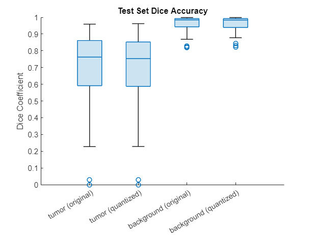
Measure the segmentation accuracy using the evaluateBreastTumorDiceAccuracy helper function. This helper function computes the Dice index between the predicted and ground truth segmentations using the dice (Image Processing Toolbox) function. The helper function is attached to the example as a supporting file.
[diceTumor,diceBackground,numTestImgs] = evaluateBreastTumorDiceAccuracy(pxdsResults,dsTest);
[diceTumorQ,diceBackgroundQ,numTestImgsQ] = evaluateBreastTumorDiceAccuracy(pxdsResultsQ,dsTest);
Visualize statistics about the Dice scores as a box chart. The middle blue line in the plot shows the median Dice index. The upper and lower bounds of the blue box indicate the 25th and 75th percentiles, respectively. Black whiskers extend to the most extreme data points that are not outliers.
figure
diceResult = [diceTumor diceTumorQ diceBackground diceBackgroundQ];
boxchart(diceResult)
title("Test Set Dice Accuracy")
xticklabels(["tumor (original)" "tumor (quantized)" ...
    "background (original)" "background (quantized)"])
ylabel("Dice Coefficient")
Investigate Behavior of Quantized Network
By using interpretability methods like Grad-CAM, you can see which parts of an input a network uses to make its predictions. You can use Grad-CAM to compare the behavior of the original network and the quantized network.
To use Grad-CAM for semantic segmentation, you must select a feature layer from which to extract the feature map and a reduction layer from which to extract the output activations. Use analyzeNetwork to determine which layers to use with Grad-CAM. In this example, you use the final ReLU layer as the feature layer and the softmax layer as the reduction layer.
analyzeNetwork(qNet)
featureLayer = "dec_relu4";
reductionlayer = "softmax-out";
classes = classNames;
Find the Grad-CAM maps for a test image. Resize the image to the size expected by the network.
testImage = preview(imds);
testImage = imresize(testImage,inputSize);
testImageGray = rgb2gray(testImage);
Segment the image using the quantized network.
segmentedImg = semanticseg(testImage,qNet);
overlayImg = labeloverlay(testImage,segmentedImg, ...
    Transparency=0.7, ...
    IncludedLabels="tumor", ...
    Colormap="hsv");
Find the Grad-CAM maps for the original and quantized networks using the gradCAM function. For each network, the function returns a map for each class showing which part of the image the network looks at for that class.
map = gradCAM(trainedNet,testImageGray,classes, ...
    ReductionLayer=reductionlayer, ...
    FeatureLayer=featureLayer);

qMap = gradCAM(qNet,testImageGray,classes, ...
    ReductionLayer=reductionlayer, ...
    FeatureLayer=featureLayer);
Plot the Grad-CAM maps for the tumor class.
figure
tiledlayout("flow",TileSpacing="compact")
nexttile
imshow(testImage)
title("Test Image")

nexttile
imshow(overlayImg)
title("Segmented Image")

nexttile
imshow(testImage)
hold on
imagesc(map(:,:,1),AlphaData=0.5)
title({"Grad-CAM for Original Model","Class: Tumor"})
hold off

nexttile
imshow(testImage)
hold on
imagesc(qMap(:,:,1),AlphaData=0.5)
title({"Grad-CAM for Quantized Model","Class: Tumor"})
hold off
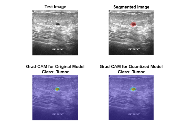
Plot the Grad-CAM maps for the background class. The Grad-CAM maps and semantic segmentation maps show similar highlighting for both classes. The Grad-CAM map for the tumor class shows that the border around the tumor is important for the classification decision of the network. Both networks might misclassify areas near the tumor boundary as part of the tumor class.
figure
tiledlayout("flow",TileSpacing="compact")
nexttile
imshow(testImage)
title("Test Image")

nexttile
imshow(overlayImg)
title("Segmented Image")

nexttile
imshow(testImage)
hold on
imagesc(map(:,:,2),AlphaData=0.5)
title(["Grad-CAM for Original Model","Class: Background"])
hold off

nexttile
imshow(testImage)
hold on
imagesc(qMap(:,:,2),AlphaData=0.5)
title(["Grad-CAM for Quantized Model","Class: Background"])
hold off

References
[1] Salehi, Seyed Sadegh Mohseni, Deniz Erdogmus, and Ali Gholipour. “Tversky Loss Function for Image Segmentation Using 3D Fully Convolutional Deep Networks.” In Machine Learning in Medical Imaging, edited by Qian Wang, Yinghuan Shi, Heung-Il Suk, and Kenji Suzuki, 10541:379–87. Cham: Springer International Publishing, 2017. https://doi.org/10.1007/978-3-319-67389-9_44.
[2] Al-Dhabyani, Walid, Mohammed Gomaa, Hussien Khaled, and Aly Fahmy. “Dataset of Breast Ultrasound Images.” Data in Brief 28 (February 2020): 104863. https://doi.org/10.1016/j.dib.2019.104863.
See Also
gradCAM | quantize | dlquantizer | calibrate
Related Topics
- Breast Tumor Segmentation from Ultrasound Using Deep Learning (Medical Imaging Toolbox)
- Quantization of Deep Neural Networks
- Quantize Residual Network Trained for Image Classification and Generate CUDA Code
- Explore Semantic Segmentation Network Using Grad-CAM
- Grad-CAM Reveals the Why Behind Deep Learning Decisions
You can also select a web site from the following list
Americas
- América Latina (Español)
- Canada (English)
- United States (English)
Europe
- Belgium (English)
- Denmark (English)
- Deutschland (Deutsch)
- España (Español)
- Finland (English)
- France (Français)
- Ireland (English)
- Italia (Italiano)
- Luxembourg (English)
- Netherlands (English)
- Norway (English)
- Österreich (Deutsch)
- Portugal (English)
- Sweden (English)
- Switzerland
- United Kingdom (English)
Asia Pacific
- Australia (English)
- India (English)
- New Zealand (English)
- 中国
- 日本Japanese (日本語)
- 한국Korean (한국어)