cwt

Continuous 1-D wavelet transform

Syntax

wt = cwt(x)

wt = cwt(x,wname)

[wt,f] = cwt(___,fs)

[wt,period] = cwt(___,ts)

[wt,f,coi] = cwt(___)

[wt,period,coi] = cwt(___,ts)

[___,coi,fb] = cwt(___)

[___,fb,scalingcfs] = cwt(___)

[___] = cwt(___,Name=Value)

cwt(___)

Description

wt = cwt(x) returns the continuous wavelet transform (CWT) of x. The CWT is obtained using the analytic Morse wavelet with the symmetry parameter, gamma ($$\gamma$$), equal to 3 and the time-bandwidth product equal to 60. cwt uses 10 voices per octave. The minimum and maximum scales are determined automatically based on the energy spread of the wavelet in frequency and time.

The cwt function uses L₁ normalization. With L₁ normalization, if you have equal amplitude oscillatory components in your data at different scales, they will have equal magnitude in the CWT. Using L₁ normalization shows a more accurate representation of the signal. See L1 Norm for CWT and Continuous Wavelet Transform of Two Complex Exponentials.

wt = cwt(x,wname) uses the analytic wavelet specified by wname to compute the CWT.

[wt,f] = cwt(___,fs) specifies the sampling frequency, fs, in hertz, and returns the scale-to-frequency conversions f in hertz. If you do not specify a sampling frequency, cwt returns f in cycles per sample.

The syntax cwt(x,fs,wname) is equivalent to cwt(x,wname,fs).

[wt,period] = cwt(___,ts) specifies the sampling period, ts, as a positive duration scalar. cwt uses ts to compute the scale-to-period conversions, period. period is an array of durations with the same Format property as ts.

[wt,f,coi] = cwt(___) returns the cone of influence, coi, in cycles per sample. Specify a sampling frequency, fs, in hertz, to return the cone of influence in hertz.

[wt,period,coi] = cwt(___,ts) returns the cone of influence, coi, as an array of durations with the same Format property as ts.

[___,coi,fb] = cwt(___) returns the filter bank used in the CWT. See cwtfilterbank.

[___,fb,scalingcfs] = cwt(___) returns the scaling coefficients for the wavelet transform.

[___] = cwt(___,Name=Value) specifies one or more additional name-value arguments. For example, wt = cwt(x,TimeBandwidth=40,VoicesPerOctave=20) specifies a time-bandwidth product of 40 and 20 voices per octave.

cwt(___) with no output arguments plots the CWT scalogram in the current figure window or specified target parent container. The scalogram is the absolute value of the CWT plotted as a function of time and frequency. Frequency is plotted on a logarithmic scale. The cone of influence showing where edge effects become significant is also plotted. Gray regions outside the dashed white line delineate regions where edge effects are significant.

For a complex-valued input signal, if you do not specify a target parent container, the function plots the positive (counterclockwise) and negative (clockwise) components in separate scalograms in the current figure window. Otherwise, the function plots the concatenation of the positive and negative components in the target parent container.

If you do not specify a sampling frequency or sampling period, the frequencies are plotted in cycles per sample. If you specify a sampling frequency, the frequencies are in hertz. If you specify a sampling period, the scalogram is plotted as a function of time and periods. If the input signal is a timetable, the scalogram is plotted as a function of time and frequency in hertz and uses the RowTimes as the basis for the time axis.

To see the time, frequency, and magnitude of a scalogram point, enable data tips in the figure axes toolbar and click the desired point in the scalogram.

Note

The cwt function clears the current figure before plotting the scalogram on it. To learn how to display the scalogram in a subplot, see Plot CWT Scalogram in Subplot.

Examples

Continuous Wavelet Transform Using Default Values

Obtain the continuous wavelet transform of a speech sample using default values.

load mtlb;
w = cwt(mtlb);

Continuous Wavelet Transform Using Specified Wavelet

Load the file mtlb. The file contains the speech sample mtlb and sample rate Fs.

load mtlb

Display the scalogram of the speech sample obtained using the analytic Morlet wavelet.

cwt(mtlb,"amor",Fs)

Compare with the scalogram obtained using the default Morse wavelet.

cwt(mtlb,Fs)

Continuous Wavelet Transform of Earthquake Data

Obtain the CWT of the Kobe earthquake data. The data are seismograph (vertical acceleration, nm/sq.sec) measurements recorded at Tasmania University, Hobart, Australia on 16 January 1995 beginning at 20:56:51 (GMT) and continuing for 51 minutes. The sampling frequency is 1 Hz.

load kobe

Plot the earthquake data.

plot((1:numel(kobe))./60,kobe)
xlabel("Time (mins)")
ylabel("Vertical Acceleration (nm/s^2)")
title("Kobe Earthquake Data")
grid on
axis tight

Obtain the CWT, frequencies, and cone of influence.

[wt,f,coi] = cwt(kobe,1);

View the scalogram, including the cone of influence.

cwt(kobe,1)

Obtain the CWT, time periods, and cone of influence by specifying a sampling period instead of a sampling frequency.

[wt,periods,coi] = cwt(kobe,minutes(1/60));

View the scalogram generated when specifying a sampling period.

cwt(kobe,minutes(1/60))

Continuous Wavelet Transform of Two Complex Exponentials

Create two complex exponentials, of different amplitudes, with frequencies of 32 and 64 Hz. The data is sampled at 1000 Hz for one second. The exponentials have disjoint support in time.

Fs = 1e3;
t = 0:1/Fs:1;
z = exp(1i*2*pi*32*t).*(t>=0.1 & t<0.3) + ...
    2*exp(-1i*2*pi*64*t).*(t>0.7);

Add complex white Gaussian noise with a standard deviation of 0.05.

wgnNoise = 0.05/sqrt(2)*(randn(size(t))+1i*randn(size(t)));
z = z+wgnNoise;

Obtain and plot the CWT using a Morse wavelet.

cwt(z,Fs)

Note the magnitudes of the complex exponential components in the colorbar are essentially their amplitudes even though they are at different scales. This is a direct result of the $$L_1$$ normalization. You can verify this by executing this script and exploring each subplot with a data cursor.

Continuous Wavelet Transform of Oceanic Eddy Data

Since R2026a

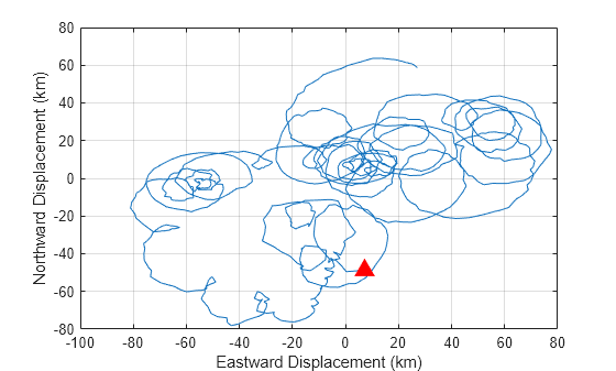
Load the NPG2006 dataset [5]. The data, which is complex valued, is the trajectory of a subsurface float trapped in an eddy. Plot the eastward and northward displacement. The triangle marks the initial position.

load npg2006
plot(npg2006.cx)
hold on
plot(npg2006.cx(1),"^",MarkerSize=11,Color="r", ...
    MarkerFaceColor="r")
hold off
grid on
xlabel("Eastward Displacement (km)")
ylabel("Northward Displacement (km)")

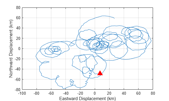
Visualize the continuous wavelet transform of the data. The sampling period is 4 hours. Because the data is complex valued, the function plots the positive (counterclockwise) and negative (clockwise) components in separate scalograms. The clockwise rotation of the float is captured in the clockwise rotary scalogram.

cwt(npg2006.cx,hours(4))

Sinusoid and Wavelet Coefficient Amplitudes

This example shows that the amplitudes of oscillatory components in a signal agree with the amplitudes of the corresponding wavelet coefficients.

Create a signal composed of two sinusoids with disjoint support in time. One sinusoid has a frequency of 32 Hz and amplitude equal to 1. The other sinusoid has a frequency of 64 Hz and amplitude equal to 2. The signal is sampled for one second at 1000 Hz. Plot the signal.

frq1 = 32;
amp1 = 1;
frq2 = 64;
amp2 = 2;

Fs = 1e3;
t = 0:1/Fs:1;
x = amp1*sin(2*pi*frq1*t).*(t>=0.1 & t<0.3)+... 
    amp2*sin(2*pi*frq2*t).*(t>0.6 & t<0.9);

plot(t,x)
grid on
xlabel("Time (sec)")
ylabel("Amplitude")
title("Signal")

Create a CWT filter bank that can be applied to the signal. Since the signal component frequencies are known, set the frequency limits of the filter bank to a narrow range that includes the known frequencies. To confirm the range, plot the magnitude frequency responses for the filter bank.

fb = cwtfilterbank(SignalLength=numel(x),SamplingFrequency=Fs,...
    FrequencyLimits=[20 100]);
freqz(fb)

Use cwt and the filter bank to plot the scalogram of the signal.

cwt(x,FilterBank=fb)

Use a data cursor to confirm that the amplitudes of the wavelet coefficients are essentially equal to the amplitudes of the sinusoidal components.

Compare Affects of Boundary Extensions on Scalogram

Since R2026a

This example shows how the different boundary extensions can affect the scalogram.

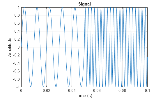
Generate a signal that consists of two sinusoids with disjoint time support. The sinusoids have different frequencies, 100 Hz and 400 Hz. The signal is sampled at 10 kHz for 1/10 of a second.

frq1 = 100;
frq2 = 400;

Fs = 10e3;
tm = 0:1/Fs:0.1-1/Fs;
len = length(tm);
brk = tm(floor(len/2)+1);

sig = sin(2*pi*frq1*tm).*(tm>=0 & tm<brk)+ ... 
    sin(2*pi*frq2*tm).*(tm>=brk & tm<=tm(end));
plot(tm,sig)
grid on
title("Signal")
xlabel("Time (s)")
ylabel("Amplitude")

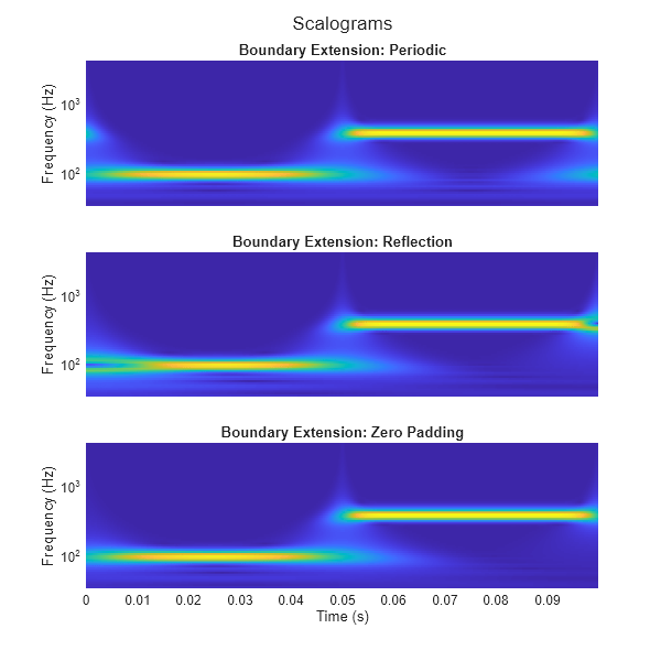
For each supported boundary extension, obtain the CWT of the signal using that extension.

[wtr,f] = cwt(sig,Fs,Boundary="reflection");
wtp = cwt(sig,Fs,Boundary="periodic");
wtz = cwt(sig,Fs,Boundary="zeropad");

Plot the scalogram of each CWT. Because different frequencies occur at the boundaries, using periodic boundary extension ("periodic") results in wrap-around effects. Using symmetric boundary extension ("reflection") creates artifacts because you are reflecting the sinusoids. For this signal, using zero padding ("zeropad") does not create boundary artifacts.

figure(Position=[0 0 600 600]);
t=tiledlayout(3,1);

nexttile
pcolor(tm,f,abs(wtp),EdgeColor="none")
xticks([])
yscale("log")
ylabel("Frequency (Hz)")
title("Boundary Extension: Periodic")

nexttile
pcolor(tm,f,abs(wtr),EdgeColor="none")
xticks([])
yscale("log")
ylabel("Frequency (Hz)")
title("Boundary Extension: Reflection")

nexttile
pcolor(tm,f,abs(wtz),EdgeColor="none")
yscale("log")
title("Boundary Extension: Zero Padding")
xlabel("Time (s)")
ylabel("Frequency (Hz)")
title(t,"Scalograms")

Using CWT Filter Bank on Multiple Time Series

This example shows how using a CWT filter bank can improve computational efficiency when taking the CWT of multiple time series.

Create a 100-by-1024 matrix x. Create a CWT filter bank appropriate for signals with 1024 samples.

x = randn(100,1024);
fb = cwtfilterbank;

Use cwt with default settings to obtain the CWT of a signal with 1024 samples. Create a 3-D array that can contain the CWT coefficients of 100 signals, each of which has 1024 samples.

cfs = cwt(x(1,:));
res = zeros(100,size(cfs,1),size(cfs,2));

Use the cwt function and take the CWT of each row of the matrix x. Display the elapsed time.

tic
for k=1:100
    res(k,:,:) = cwt(x(k,:));
end
toc

Elapsed time is 0.928160 seconds.

Now use the wt object function of the filter bank to take the CWT of each row of x. Display the elapsed time.

tic
for k=1:100
    res(k,:,:) = wt(fb,x(k,:));
end
toc

Elapsed time is 0.393524 seconds.

CUDA Code from CWT

This example shows how to generate a MEX file to perform the continuous wavelet transform (CWT) using generated CUDA® code.

First, ensure that you have a CUDA-enabled GPU and the NVCC compiler. See The GPU Environment Check and Setup App (GPU Coder) to ensure you have the proper configuration.

Create a GPU coder configuration object.

cfg = coder.gpuConfig("mex");

Generate a signal of 100,000 samples at 1,000 Hz. The signal consists of two cosine waves with disjoint time supports.

t = 0:.001:(1e5*0.001)-0.001;
x = cos(2*pi*32*t).*(t > 10 & t<=50)+ ...
    cos(2*pi*64*t).*(t >= 60 & t < 90)+ ...
    0.2*randn(size(t));

Cast the signal to use single precision. GPU calculations are often more efficiently done in single precision. You can however also generate code for double precision if your NVIDIA® GPU supports it.

x = single(x);

Generate the GPU MEX file and a code generation report. To allow generation of the MEX file, you must specify the properties (class, size, and complexity) of the three input parameters:

• coder.typeof(single(0),[1 1e5]) specifies a row vector of length 100,000 containing real single values.

• coder.typeof('c',[1 inf]) specifies a character array of arbitrary length.

• coder.typeof(0) specifies a real double value.

sig = coder.typeof(single(0),[1 1e5]);
wav = coder.typeof('c',[1 inf]);
sfrq = coder.typeof(0);
codegen cwt -config cfg -args {sig,wav,sfrq} -report

Code generation successful: View report

The -report flag is optional. Using -report generates a code generation report. In the Summary tab of the report, you can find a GPU code metrics link, which provides detailed information such as the number of CUDA kernels generated and how much memory was allocated.

Run the MEX file on the data and plot the scalogram. Confirm the plot is consistent with the two disjoint cosine waves.

[cfs,f] = cwt_mex(x,'morse',1e3);
image("XData",t,"YData",f,"CData",abs(cfs),"CDataMapping","scaled")
set(gca,"YScale","log")
axis tight
xlabel("Time (Seconds)")
ylabel("Frequency (Hz)")
title("Scalogram of Two-Tone Signal")

Run the CWT command above without appending the _mex. Confirm the MATLAB® and the GPU MEX scalograms are identical.

[cfs2,f2] = cwt(x,'morse',1e3);
max(abs(cfs2(:)-cfs(:)))

ans = single
    7.3380e-07

Change Default Frequency Axis Labels

This example shows how to change the default frequency axis labels for the CWT when you obtain a plot with no output arguments.

Create two sine waves with frequencies of 32 and 64 Hz. The data is sampled at 1000 Hz. The two sine waves have disjoint support in time. Add white Gaussian noise with a standard deviation of 0.05. Obtain and plot the CWT using the default Morse wavelet.

Fs = 1e3;
t = 0:1/Fs:1;
x = cos(2*pi*32*t).*(t>=0.1 & t<0.3)+sin(2*pi*64*t).*(t>0.7);
wgnNoise = 0.05*randn(size(t));
x = x+wgnNoise;
cwt(x,1000)

The plot uses a logarithmic frequency axis because frequencies in the CWT are logarithmic. In MATLAB, logarithmic axes are in powers of 10 (decades). You can use cwtfreqbounds to determine what the minimum and maximum wavelet bandpass frequencies are for a given signal length, sampling frequency, and wavelet.

[minf,maxf] = cwtfreqbounds(numel(x),1000);

You see that by default MATLAB has placed frequency ticks at 10 and 100 because those are the powers of 10 between the minimum and maximum frequencies. If you wish to add more frequency axis ticks, you can obtain a logarithmically spaced set of frequencies between the minimum and maximum frequencies using the following.

numfreq = 10;
freq = logspace(log10(minf),log10(maxf),numfreq);

Next, get the handle to the current axes and replace the frequency axis ticks and labels with the following.

AX = gca;
AX.YTickLabelMode = "auto";
AX.YTick = freq;

In the CWT, frequencies are computed in powers of two. To create the frequency ticks and tick labels in powers of two, you can do the following.

newplot
cwt(x,1000)
AX = gca;
freq = 2.^(round(log2(minf)):round(log2(maxf)));
AX.YTickLabelMode = "auto";
AX.YTick = freq;

Change Scalogram Coloration

This example shows how to scale scalogram values by maximum absolute value at each level for plotting.

Load in a signal and display the default scalogram. Change the colormap to pink(240).

load noisdopp
cwt(noisdopp)
colormap(pink(240))

Take the CWT of the signal and obtain the wavelet coefficients and frequencies.

[cfs,frq] = cwt(noisdopp);

To efficiently find the maximum value of the coefficients at each frequency (level), first transpose the absolute value of the coefficients. Find the minimum value at every level. At each level, subtract the level's minimum value.

tmp1 = abs(cfs);
t1 = size(tmp1,2);
tmp1 = tmp1';
minv = min(tmp1);
tmp1 = (tmp1-minv(ones(1,t1),:));

Find the maximum value at every level of tmp1. For each level, divide every value by the maximum value at that level. Multiply the result by the number of colors in the colormap. Set equal to 1 all zero entries. Transpose the result.

maxv = max(tmp1);
maxvArray = maxv(ones(1,t1),:);
indx = maxvArray<eps;
tmp1 = 240*(tmp1./maxvArray);
tmp2 = 1+fix(tmp1);
tmp2(indx) = 1;
tmp2 = tmp2';

Display the result. The scalogram values are now scaled by the maximum absolute value at each level. Frequencies are displayed on a linear scale.

t = 0:length(noisdopp)-1;
pcolor(t,frq,tmp2)
shading interp
xlabel("Time (Samples)")
ylabel("Normalized Frequency (cycles/sample)")
title("Scalogram Scaled By Level")
colormap(pink(240))
colorbar

Changing the Time-Bandwidth Product

This example shows that increasing the time-bandwidth product $$P^2$$ of the Morse wavelet creates a wavelet with more oscillations under its envelope. Increasing $$P^2$$ narrows the wavelet in frequency.

Create two filter banks. One filter bank has the default TimeBandwidth value of 60. The second filter bank has a TimeBandwidth value of 10. The SignalLength for both filter banks is 4096 samples.

sigLen = 4096;
fb60 = cwtfilterbank(SignalLength=sigLen);
fb10 = cwtfilterbank(SignalLength=sigLen,TimeBandwidth=10);

Obtain the time-domain wavelets for the filter banks.

[psi60,t] = wavelets(fb60);
[psi10,~] = wavelets(fb10);

Use the scales function to find the mother wavelet for each filter bank.

sca60 = scales(fb60);
sca10 = scales(fb10);
[~,idx60] = min(abs(sca60-1));
[~,idx10] = min(abs(sca10-1));
m60 = psi60(idx60,:);
m10 = psi10(idx10,:);

Since the time-bandwidth product is larger for the fb60 filter bank, verify the m60 wavelet has more oscillations under its envelope than the m10 wavelet.

tiledlayout(2,1)
nexttile
plot(t,abs(m60))
grid on
hold on
plot(t,real(m60))
plot(t,imag(m60))
hold off
xlim([-30 30])
legend("abs(m60)","real(m60)","imag(m60)")
title("TimeBandwidth = 60")
nexttile
plot(t,abs(m10))
grid on
hold on
plot(t,real(m10))
plot(t,imag(m10))
hold off
xlim([-30 30])
legend("abs(m10)","real(m10)","imag(m10)")
title("TimeBandwidth = 10")

Align the peaks of the m60 and m10 magnitude frequency responses. Verify the frequency response of the m60 wavelet is narrower than the frequency response for the m10 wavelet.

cf60 = centerFrequencies(fb60);
cf10 = centerFrequencies(fb10);

m60cFreq = cf60(idx60);
m10cFreq = cf10(idx10);

freqShift = 2*pi*(m60cFreq-m10cFreq);
x10 = m10.*exp(1j*freqShift*(-sigLen/2:sigLen/2-1));

figure
plot([abs(fft(m60)).' abs(fft(x10)).'])
grid on
legend("Time-Bandwidth = 60","Time-Bandwidth = 10")
title("Magnitude Frequency Responses")

Plot CWT Scalogram in Subplot

This example shows how to plot the CWT scalogram in a figure subplot.

Load the speech sample. The data is sampled at 7418 Hz. Plot the default CWT scalogram.

load mtlb
cwt(mtlb,Fs)

Obtain the CWT of the signal, and the scale-to-frequency conversions of the CWT.

[cfs,frq] = cwt(mtlb,Fs);

The cwt function sets the time and frequency axes in the scalogram. Create a vector representing the sample times.

tms = (0:numel(mtlb)-1)/Fs;

In a new figure, plot the original signal in the upper subplot and the scalogram in the lower subplot. Plot the frequencies on a logarithmic scale.

figure
tiledlayout(2,1)
nexttile
plot(tms,mtlb)
axis tight
title("Signal and Scalogram")
xlabel("Time (s)")
ylabel("Amplitude")
nexttile
surface(tms,frq,abs(cfs))
axis tight
shading flat
xlabel("Time (s)")
ylabel("Frequency (Hz)")
set(gca,"yscale","log")

Plot CWT Scalogram in Target Axes and Panel Container

Since R2026a

Plot the CWT scalogram for four signals in the specified target axes and panel containers.

Plot CWT Scalogram in Target Axes

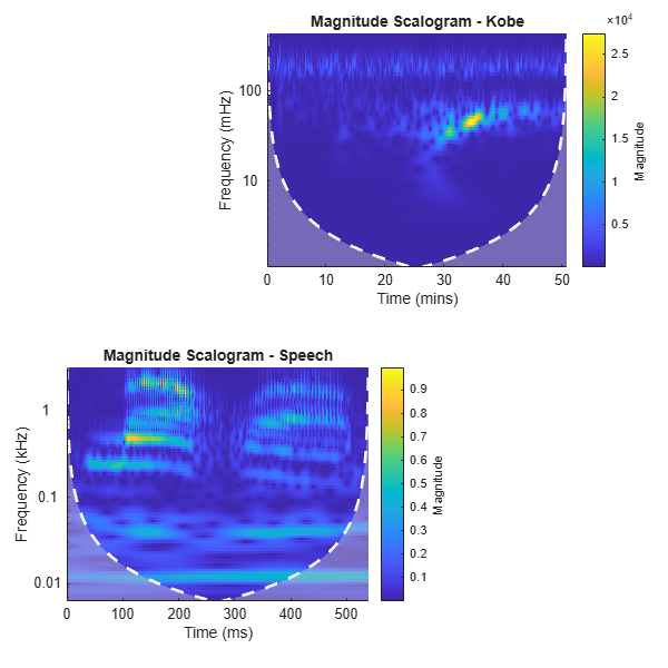
Load the speech sample. The sample rate is 7418 Hz. Load the Kobe earthquake data. The sample rate is 1 Hz.

load mtlb
FsSpeech = 7418;
load kobe
FsKobe = 1;

Create two axes in the southwestern and northeastern corners of a new figure window.

fig = figure(Position=[100 100 600 600]);
ax1 = axes(fig,Position=[0.1 0.1 0.55 0.35]);
ax2 = axes(fig,Position=[0.4 0.6 0.55 0.35]);

Plot the CWT scalogram of the speech and Kobe data in the southwestern and northeastern axes of the figure, respectively.

cwt(mtlb,FsSpeech,Parent=ax1)
title(ax1,"Magnitude Scalogram - Speech")
cwt(kobe,FsKobe,Parent=ax2)
title(ax2,"Magnitude Scalogram - Kobe")

Plot CWT Scalogram in Target UI Axes

Load the noisy Doppler signal.

load noisdopp

Create an axes in the southwestern corner of a new UI figure window.

uif = uifigure(Position=[100 100 720 540]);
ax3 = uiaxes(uif,Position=[60 70 400 200]);

Plot the CWT scalogram of the noisy Doppler signal on the figure axes.

cwt(noisdopp,Parent=ax3)
title(ax3,"Magnitude Scalogram - Doppler")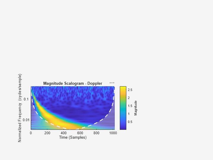

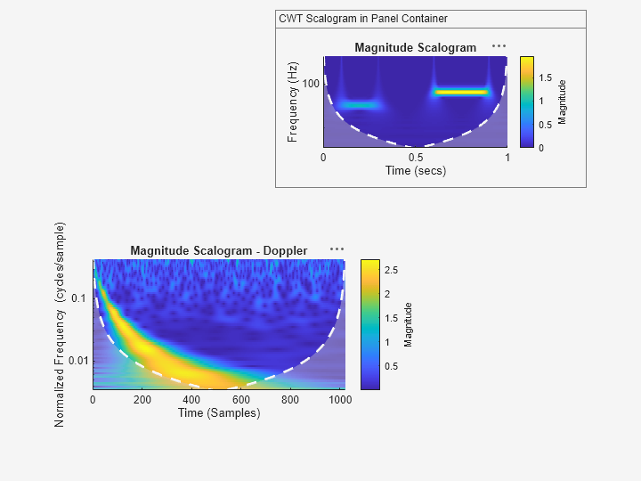
Plot CWT Scalogram in Target Panel Container

Create a signal composed of two sinusoids with disjoint support in time. One sinusoid has a frequency of 32 Hz and amplitude equal to 1. The other sinusoid has a frequency of 64 Hz and amplitude equal to 2. Sample the signal for one second at 1000 Hz.

frq1 = 32;
amp1 = 1;
frq2 = 64;
amp2 = 2;

Fs = 1e3;
t = 0:1/Fs:1;
x = amp1*sin(2*pi*frq1*t).*(t>=0.1 & t<0.3)+... 
    amp2*sin(2*pi*frq2*t).*(t>0.6 & t<0.9);

Add a panel container in the northeastern corner of the UI figure window.

p = uipanel(uif,Position=[310 330 350 200], ...
    Title="CWT Scalogram in Panel Container");

Plot the CWT scalogram of the sinusoidal signal on the panel container.

cwt(x,Fs,Parent=p)

Plot CWT Scalogram of Complex-Valued Signal in Target Axes

Since R2026a

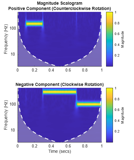
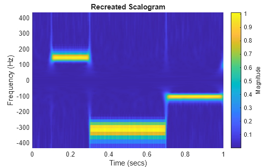
Generate a signal sampled at 1 kHz for one second. The signal consists of three complex-valued sinusoids and white noise. Each sinusoid has a different frequency. Two frequencies are negative. The sinusoids have disjoint time support.

Fs = 1e3;
t = 0:1/Fs:1;
z = exp(1i*2*pi*150*t).*(t>=0.1 & t<0.3) + ...
    exp(-1i*2*pi*300*t).*(t>=0.3 & t<0.7) + ...
    exp(-1i*2*pi*100*t).*(t>0.7);

wgnNoise = 0.05/sqrt(2)*(randn(size(t)) + ...
    1i*randn(size(t)));
sig = z + wgnNoise;

Plot the scalogram of the signal without specifying a target parent container. Because the signal is complex-valued, the function plots the positive and negative components in separate scalograms. The function uses a log scale for the frequency.

cwt(sig,Fs)

Create an axes in a new figure window. Use the Parent name-value argument syntax to plot the scalogram in the axes. Also obtain the CWT coefficients and frequencies. The negative component corresponds to the negative frequencies in the plot. The function uses a linear scale for the frequency.

fig = figure;
ax = axes(fig,Position=[0.1 0.1 0.5 0.6]);
[cfs,f] = cwt(sig,Fs,Parent=ax);

The function returns the CWT coefficients in a 3-D array. The first page corresponds to the positive (counterclockwise) component and the second page corresponds to the negative (clockwise) component.

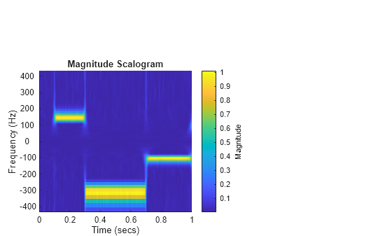
You can use the coefficients and frequencies to recreate the target axes plot in a new figure. Rearrange and concatenate the two pages.

flpdp = flip(cfs(:,:,2));
cfs2 = cat(1,cfs(:,:,1),flpdp);

Rearrange and concatenate the frequency vector such that the frequencies range from positive to negative values.

flpdv = flip(-f);
f2 = cat(1,f,flpdv);

Add an axes ax2 to a new figure. Use the surf function to plot the absolute value of the concatenated coefficients on ax2.

ax2 = axes(figure);
surf(ax2,t,f2,abs(cfs2),EdgeColor="none")
view(ax2,[0,90])
axis(ax2,"tight")
set(ax2,YDir="normal")
xlabel(ax2,"Time (secs)")
ylabel(ax2,"Frequency (Hz)")
c = colorbar(ax2);
c.Label.String = "Magnitude";
title(ax2,"Recreated Scalogram")

Specifying Sample Period and Parent Name-Value Argument for Complex-Valued Signal

Since R2026a

Load the NPG2006 data set. The complex-valued data is the trajectory of a subsurface float trapped in an eddy. The sample period is four hours. Plot the eastward and northward displacement. The triangle marks the initial position.

load npg2006
sig = npg2006.cx;
plot(sig)
hold on
plot(npg2006.cx(1),"^",MarkerSize=11,Color="r", ...
    MarkerFaceColor=[1 0 0 ])
hold off
grid on
xlabel("Eastward Displacement (km)")
ylabel("Northward Displacement (km)")

Create an axes in a new UI figure window. Plot the scalogram on the axes using the Parent name-value argument and also obtain the periods p and cone of influence coi. If you specify a sample period in hours, then p and coi are also duration arrays in units of hours. Note that although p and coi are duration arrays, if you call cwt with a target parent container and a complex-valued signal, the function plots the scalogram with respect to frequencies.

uif = uifigure(Position=[100 100 720 540]);
axf = uiaxes(uif,Position=[15 105 575 400]);

[cfs,p,coi] = cwt(sig,hours(4),Parent=axf);

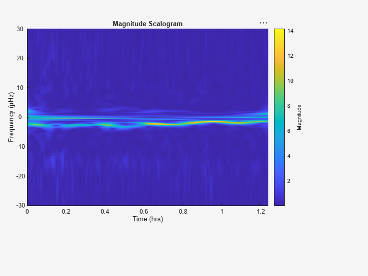
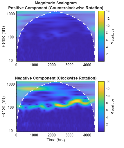
To visualize the clockwise and counterclockwise components of the scalogram in terms of periods, use cwt without specifying a target parent container or output arguments.

figure
cwt(sig,hours(4))

Input Arguments

x — Input signal

vector | timetable

Input signal, specified as a vector or a single-variable regularly sampled timetable. The input x must have at least four samples.

Data Types: single | double
Complex Number Support: Yes

wname — Analytic wavelet

"morse" (default) | "amor" | "bump"

Analytic wavelet used to compute the CWT. Valid options for wname are "morse", "amor", and "bump", which specify the Morse, Morlet (Gabor), and bump wavelet, respectively.

The default Morse wavelet has symmetry parameter gamma ($$\gamma$$) equal to 3 and time-bandwidth product equal to 60.

Data Types: char | string

fs — Sampling frequency

positive scalar

Sampling frequency in hertz, specified as a positive scalar. If you specify fs, then you cannot specify ts. If x is a timetable, you cannot specify fs. fs is determined from the RowTimes of the timetable.

Data Types: single | double

ts — Sampling period

scalar duration

Sampling period, also known as the time duration, specified as a scalar duration. Valid durations are years, days, hours, minutes, and seconds. You cannot use calendar durations. If you specify ts, then you cannot specify fs. If x is a timetable, you cannot specify ts. ts is determined from the RowTimes of the timetable when you set the PeriodLimits name-value argument.

Example: wt = cwt(x,hours(12))

Data Types: duration

Name-Value Arguments

Specify optional pairs of arguments as Name1=Value1,...,NameN=ValueN, where Name is the argument name and Value is the corresponding value. Name-value arguments must appear after other arguments, but the order of the pairs does not matter.

Example: wt = cwt(x,"bump",VoicesPerOctave=10) returns the CWT of x using the bump wavelet and 10 voices per octave.

FrequencyLimits — Frequency limits

two-element scalar vector

Frequency limits to use in the CWT, specified as a two-element vector with positive strictly increasing entries.

• The first element specifies the lowest peak passband frequency and must be greater than or equal to the product of the wavelet peak frequency in hertz and two time standard deviations divided by the signal length.

• The second element specifies the highest peak passband frequency and must be less than or equal to the Nyquist frequency.

• The base-2 logarithm of the ratio of the upper frequency limit, freqMax, to the lower frequency limit, freqMin, must be greater than or equal to 1/NV, where NV is the number of voices per octave:

  log2(freqMax/freqMin) ≥ 1/NV.

For complex-valued signals, (-1) × flimits is used for the anti-analytic part, where flimits is the vector specified by FrequencyLimits.

Note

If you specify frequency limits outside the permissible range, cwt truncates the limits to the minimum and maximum valid values. Use cwtfreqbounds to determine frequency limits for different parameterizations of the CWT.

Example: wt = cwt(x,1000,VoicesPerOctave=10,FrequencyLimits=[80 90])

Data Types: double

PeriodLimits — Period limits

two-element duration array

Period limits to use in the CWT, specified as a two-element duration array with strictly increasing positive entries.

• The first element must be greater than or equal to 2 × ts, where ts is the sampling period.

• The maximum period cannot exceed the signal length divided by the product of two time standard deviations of the wavelet and the wavelet peak frequency.

• The base-2 logarithm of the ratio of the minimum period, minP, to the maximum period, maxP, must be less than or equal to -1/NV, where NV is the number of voices per octave:

  log2(pMin/pMax) ≤ -1/NV.

For complex-valued signals, (-1) × plimits is used for the anti-analytic part, where plimits is the vector specified by PeriodLimits.

Note

If you specify period limits outside the permissible range, cwt truncates the limits to the minimum and maximum valid values. Use cwtfreqbounds to determine period limits for different parameterizations of the wavelet transform.

Example: wt = cwt(x,seconds(0.1),VoicesPerOctave=10,PeriodLimits=[seconds(0.2) seconds(3)])

Data Types: duration

VoicesPerOctave — Number of voices per octave

10 (default) | integer from 1 to 48

Number of voices per octave to use for the CWT, specified as an integer from 1 to 48. The CWT scales are discretized using the specified number of voices per octave. The energy spread of the wavelet in frequency and time automatically determines the minimum and maximum scales.

TimeBandwidth — Time-bandwidth product of the Morse wavelet

60 (default) | scalar greater than or equal to 3 and less than or equal to 120

Time-bandwidth product of the Morse wavelet, specified as a scalar greater than or equal to 3 and less than or equal to 120. The symmetry parameter, gamma ($$\gamma$$), is fixed at 3. Wavelets with larger time-bandwidth products have larger spreads in time and narrower spreads in frequency. The standard deviation of the Morse wavelet in time is approximately sqrt(TimeBandwidth/2). The standard deviation of the Morse wavelet in frequency is approximately 1/2 × sqrt(2/TimeBandwidth).

By default, the cwt function uses frequency limits that depend on the wavelet. The limits are based on the energy spread of the wavelet in frequency and time. If you change the time-bandwidth product, you also change the default frequency limits. (Similarly, you change the default period limits.) To compare the continuous wavelet transforms of a signal obtained using different time-bandwidth products, set FrequencyLimits to the same value for the different transforms.

If you specify TimeBandwidth, you cannot specify WaveletParameters. To specify both the symmetry and time-bandwidth product, use WaveletParameters instead.

In the notation of Morse Wavelets, TimeBandwidth is P².

WaveletParameters — Symmetry and time-bandwidth product of the Morse wavelet

[3 60] (default) | two-element vector of scalars

Symmetry and time-bandwidth product of the Morse wavelet, specified as a two-element vector of scalars. The first element is the symmetry, $$\gamma$$, which must be greater than or equal to 1. The second element is the time-bandwidth product, which must be greater than or equal to $$\gamma$$. The ratio of the time-bandwidth product to $$\gamma$$ cannot exceed 40.

When $$\gamma$$ is equal to 3, the Morse wavelet is perfectly symmetric in the frequency domain and the skewness is 0. When $$\gamma$$ is greater than 3, the skewness is positive. When $$\gamma$$ is less than 3, the skewness is negative. For more information, see Morse Wavelets.

By default, the cwt function uses frequency limits that depend on the wavelet. The limits are based on the energy spread of the wavelet in frequency and time. If you change the wavelet parameters, you also change the default frequency limits. (Similarly, you change the default period limits.) To compare the continuous wavelet transforms of a signal obtained using different wavelet parameters, set FrequencyLimits to the same value for the different transforms.

If you specify WaveletParameters, you cannot specify TimeBandwidth.

Boundary — Boundary extension

"reflection" (default) | "periodic" | "zeropad"

Since R2026a

Boundary extension of signal, specified as one of these values:

• "reflection" — Extend the signal symmetrically at the left and right boundaries.

• "periodic" — Extend the signal periodically.

• "zeropad" — Extend the signal at the left and right boundaries by zero padding.

If you specify "reflection" or "zeropad", the cwt function internally extends the input signal to twice its original size. On the other hand, if you specify "periodic", the function treats the signal as periodic. The signal size does not change.

Note

If you want to invert the CWT using icwt with scaling coefficients and approximate synthesis filters, set Boundary to "periodic".

FilterBank — CWT filter bank

cwtfilterbank object

CWT filter bank to use to compute the CWT, specified as a cwtfilterbank object. If you set FilterBank, you cannot specify any other options. All options for the computation of the CWT are defined as properties of the filter bank. For more information, see cwtfilterbank.

If x is a timetable, the sampling frequency or sampling period in fb must agree with the sampling frequency or sampling period determined by the RowTimes of the timetable.

Example: wt = cwt(x,FilterBank=cfb)

Parent — Target parent container

[] (default) | Axes object | UIAxes object | Panel object

Since R2026a

Target parent container, specified as an Axes object, a UIAxes object, or a Panel object.

If you specify Parent=P and P is nonempty, the cwt function plots the scalogram as a function of time and frequency on the specified target parent container even if you specify output arguments. See Plot CWT Scalogram in Target Axes and Panel Container.

If the input signal is complex-valued, cwt concatenates the positive (counterclockwise) and negative (clockwise) components and plots the result on the target parent. The negative component corresponds to the negative frequencies in the plot. See Plot CWT Scalogram of Complex-Valued Signal in Target Axes. You can obtain the same visualization for the scalogram of a complex-valued signal in the Wavelet Time-Frequency Analyzer app. To do so, clear the Separate positive and negative components for complex signals check box under Preferences on the Analyzer tab.

For a complex-valued signal, if you specify a sampling period and a nonempty parent, cwt uses frequencies in the plot. However, the function still returns the relevant output arguments as duration arrays. See Specifying Sample Period and Parent Name-Value Argument for Complex-Valued Signal.

For more information about target containers and the parent-child relationship in MATLAB^® graphics, see Graphics Object Hierarchy. For more information about using Parent in UIAxes and Panel objects to design apps, see Plot Spectral Representations of Signal in App Designer.

Output Arguments

wt — Continuous wavelet transform

matrix

Continuous wavelet transform, returned as a matrix of complex values. By default, cwt uses the analytic Morse (3,60) wavelet, where 3 is the symmetry and 60 is the time-bandwidth product. cwt uses 10 voices per octave.

• If x is real-valued, wt is an Na-by-N matrix, where Na is the number of scales, and N is the number of samples in x.

• If x is complex-valued, wt is a 3-D matrix, where the first page is the CWT for the positive scales (analytic part or counterclockwise component) and the second page is the CWT for the negative scales (anti-analytic part or clockwise component).

The minimum and maximum scales are determined automatically based on the energy spread of the wavelet in frequency and time. See Algorithms for information on how the scales are determined.

Data Types: single | double

f — Scale-to-frequency conversions

vector

Scale-to-frequency conversions of the CWT, returned as a vector. If you specify a sampling frequency, fs, then f is in hertz. If you do not specify fs, cwt returns f in cycles per sample. If the input x is complex, the scale-to-frequency conversions apply to both pages of wt.

period — Scale-to-period conversions

array

Scale-to-period conversions, returned as an array of durations with the same Format property as ts. Each row corresponds to a period. If the input x is complex, the scale-to-period conversions apply to both pages of wt.

coi — Cone of influence

array of real numbers | array of durations

Cone of influence for the CWT. If you specify a sampling frequency, fs, the cone of influence is in hertz. If you specify a scalar duration, ts, the cone of influence is an array of durations with the same Format property as ts. If the input x is complex, the cone of influence applies to both pages of wt.

The cone of influence indicates where edge effects occur in the CWT. Due to the edge effects, give less credence to areas that are outside or overlap the cone of influence. For additional information, see Boundary Effects and the Cone of Influence.

fb — CWT filter bank

cwtfilterbank object

CWT filter bank used in the CWT, returned as a cwtfilterbank object. See cwtfilterbank.

scalingcfs — Scaling coefficients

real- or complex-valued vector

Scaling coefficients for the CWT, returned as a real- or complex-valued vector. The length of scalingcfs is equal to the length of the input x.

More About

Analytic Wavelets

Analytic wavelets are complex-valued wavelets whose Fourier transform vanish for negative frequencies. Analytic wavelets are a good choice when doing time-frequency analysis with the CWT. Because the wavelet coefficients are complex-valued, the coefficients provide phase and amplitude information of the signal being analyzed. Analytic wavelets are well suited for studying how the frequency content in real world nonstationary signals evolves as a function of time.

Analytic wavelets are almost exclusively based on rapidly decreasing functions. If $$\psi (t)$$ is an analytic rapidly decreasing function in time, then its Fourier transform $$\widehat{\psi }(\omega )$$ is a rapidly decreasing function in frequency and is small outside of some interval $$\alpha <\omega <\beta$$ where $$0<\alpha <\beta$$. Orthogonal and biorthogonal wavelets are typically designed to have compact support in time. Wavelets with compact support in time have relatively poorer energy concentration in frequency than wavelets which rapidly decrease in time. Most orthogonal and biorthogonal wavelets are not symmetric in the Fourier domain.

If your goal is to obtain a joint time-frequency representation of your signal, we recommend you use cwt or cwtfilterbank. Both functions support the following analytic wavelets:

• Morse Wavelet Family (default)

• Analytic Morlet (Gabor) Wavelet

• Bump Wavelet

For more information regarding Morse wavelets, see Morse Wavelets. In the Fourier domain, in terms of angular frequency:

• The analytic Morlet is defined as

  

  where is the indicator function of the interval [0,∞).

• The bump wavelet is defined as

  

  where ϵ = 2.2204×10^-16.

If you want to do time-frequency analysis using orthogonal or biorthogonal wavelets, we recommend modwpt.

When using wavelets for time-frequency analysis, you usually convert scales to frequencies or periods to interpret results. cwt and cwtfilterbank do the conversion. You can obtain the corresponding scales associated by using scales on the optional cwt output argument fb.

For guidance on how to choose the wavelet that is right for your application, see Choose a Wavelet.

Tips

• The syntax for the old cwt function continues to work but is no longer recommended. Use the current version of cwt. Both the old and current versions use the same function name. The inputs to the function determine automatically which version is used. See cwt function syntax has changed.

• When performing multiple CWTs, for example inside a for-loop, the recommended workflow is to first create a cwtfilterbank object and then use the wt object function. This workflow minimizes overhead and maximizes performance. See Using CWT Filter Bank on Multiple Time Series.

Algorithms

Minimum Scale

For the analytic wavelets supported by the cwt function, the Fourier transforms are real valued and equivalent to the magnitude frequency response (see Analytic Wavelets). The wavelet filters the cwt function uses are normalized so that the peak magnitudes for all passbands are approximately equal to 2. This is so that a unit-magnitude oscillation in the data shows up with a scalogram magnitude equal to 1.

Let $$\widehat{\psi }(\omega )$$ denote the mother wavelet in the Fourier domain. For a fixed real-valued scalar c between 0 and 1, there exists a frequency ξ such that

$$\widehat{\psi }(\xi )=2c.$$

The minimum scale $$s_0$$ is $$\xi /\pi$$.

By default, the cwt function sets the fraction of the peak magnitude at the Nyquist frequency at 50% (c equals 0.5) for the Morse wavelet and 10% (c equals 0.1) for the analytic Morlet and bump wavelets. You can change the fraction by changing the frequency or period limits to use in the CWT. For more information, see cwtfreqbounds and, in particular, the Cutoff name-value argument. See also the cwtfilterbank object function scales.

Maximum Scale

The cwt function uses the energy spread of the wavelet in time to determine the maximum scale.

To determine the maximum scale, the cwt function first obtains $${\sigma }_t$$, the time standard deviation of the wavelet. If a wavelet has a time standard deviation of $${\sigma }_t$$, then dilating that wavelet by $$s$$ gives a standard deviation of $$s{\sigma }_t$$.

The maximum scale is the value $$s$$ such that $$2s{\sigma }_t=N$$, where N is the signal length. The cwt function constrains the largest scale to be that value so that two time standard deviations of the wavelet span the data length. This ensures that at the largest scale, the wavelet oscillates and that cwt uses a valid wavelet.

Analytic expressions for the time standard deviation of the Morse wavelet exist. For the bump and analytic Morlet wavelets, the cwt function estimates the standard deviation of the mother wavelet in time by obtaining its inverse Fourier transform, normalizing it to be a valid probability density function, and then obtaining the square root of the second central moment.

Scales and Voices Per Octave

Wavelet transform scales are powers of 2 and are denoted by $$s_0{\left(2^{\frac{1}{NV}}\right)}^j$$. NV is the number of voices per octave, and j ranges from 0 to the largest scale. For a specific small scale, $$s_0$$:

$$s_0{\left(2^{\frac{1}{NV}}\right)}^j\le \frac{N}{2{\sigma }_t}$$

Converting to base-2 logarithm:

$$j{\log }_2\left(2^{\frac{1}{NV}}\right)\le {\log }_2\left(\frac{N}{2{\sigma }_t{s}_0}\right)$$

$$j\le NV{\log }_2\left(\frac{N}{2{\sigma }_t{s}_0}\right)$$

Therefore, the maximum scale is

$$s_0{\left(2^{\frac{1}{NV}}\right)}^{floor\left(NV{\log }_2\left(\frac{N}{2{\sigma }_t{s}_0}\right)\right)}$$

L₁ Norm for CWT

In integral form, the CWT preserves energy. However, when you implement the CWT numerically, energy is not preserved. In this case, regardless of the normalization you use, the CWT is not an orthonormal transform. The cwt function uses L₁ normalization.

Wavelet transforms commonly use L₂ normalization of the wavelet. For the L₂ norm, dilating a signal by 1/s, where s is greater than 0, is defined as follows:

$${\Vert x\left(\frac{t}{s}\right)\Vert }_2^2=s{\Vert x\left(t\right)\Vert }_2^2$$

The energy is now s times the original energy. When included in the Fourier transform, multiplying by $$\raisebox{1ex}{$1$}\!\left/ \!\raisebox{-1ex}{$\sqrt{s}$}\right.$$ produces different weights being applied to different scales, so that the peaks at higher frequencies are reduced more than the peaks at lower frequencies.

In many applications, L₁ normalization is better. The L₁ norm definition does not include squaring the value, so the preserving factor is 1/s instead of $$\raisebox{1ex}{$1$}\!\left/ \!\raisebox{-1ex}{$\sqrt{s}$}\right.$$. Instead of high-frequency amplitudes being reduced as in the L₂ norm, for L₁ normalization, all frequency amplitudes are normalized to the same value. Therefore, using the L₁ norm shows a more accurate representation of the signal. See example Continuous Wavelet Transform of Two Complex Exponentials.

References

[1] Lilly, J. M., and S. C. Olhede. “Generalized Morse Wavelets as a Superfamily of Analytic Wavelets.” IEEE Transactions on Signal Processing 60, no. 11 (November 2012): 6036–6041. https://doi.org/10.1109/TSP.2012.2210890.

[2] Lilly, J.M., and S.C. Olhede. “Higher-Order Properties of Analytic Wavelets.” IEEE Transactions on Signal Processing 57, no. 1 (January 2009): 146–160. https://doi.org/10.1109/TSP.2008.2007607.

[3] Lilly, J. M. jLab: A data analysis package for MATLAB, version 1.6.2. 2016. http://www.jmlilly.net/jmlsoft.html.

[4] Lilly, Jonathan M. “Element Analysis: A Wavelet-Based Method for Analysing Time-Localized Events in Noisy Time Series.” Proceedings of the Royal Society A: Mathematical, Physical and Engineering Sciences 473, no. 2200 (April 30, 2017): 20160776. https://doi.org/10.1098/rspa.2016.0776.

[5] Lilly, J. M., and J.-C. Gascard. “Wavelet Ridge Diagnosis of Time-Varying Elliptical Signals with Application to an Oceanic Eddy.” Nonlinear Processes in Geophysics 13, no. 5 (September 14, 2006): 467–83. https://doi.org/10.5194/npg-13-467-2006.

Extended Capabilities

GPU Code Generation

Generate CUDA® code for NVIDIA® GPUs using GPU Coder™.

Usage notes and limitations:

• To generate code, three input arguments are required: input signal, sample rate, and wavelet name.

• Timetable input signal is not supported.

• Only analytic Morse ("morse") and Morlet ("amor") wavelets are supported. You must specify the wavelet name as a compile-time constant. Use coder.Constant (MATLAB Coder)

• You must specify the value of Boundary as a compile-time constant. (since R2026a)

• The sampling period (ts) is not supported.

• These name-value arguments are not supported: PeriodLimits name-value argument, NumOctave name-value argument, FilterBank, and Parent.

• Scaling coefficient output and filter bank output are not supported.

• Plotting is not supported.

GPU Arrays

Accelerate code by running on a graphics processing unit (GPU) using Parallel Computing Toolbox™.

The cwt function fully supports GPU arrays. To run the function on a GPU, specify the input data as a gpuArray (Parallel Computing Toolbox). For more information, see Run MATLAB Functions on a GPU (Parallel Computing Toolbox).

Version History

Introduced in R2016b

R2026a: Create Plot Live Editor Task: Visualize continuous wavelet transform function output

You can now use the Create Plot Live Editor task to interactively visualize the output of the cwt function. You can select different chart types and set optional parameters. The task also automatically generates code that becomes part of your live script. For more information, see Create Plot.

R2026a: Visualize CWT scalogram in specified parent target containers

The cwt function supports plotting the scalogram in a parent axes or panel container using the Parent name-value argument.

R2026a: cwt supports zero-padded extension with new Boundary name-value argument

The cwt function now supports zero padding as a boundary extension mode. To specify an extension mode, use the new name-value argument Boundary. In addition to supporting zero padding, this new name-value argument makes cwt more consistent with other wavelet transform APIs, such as cwtfilterbank and dwpt.

R2026a: ExtendSignal name-value argument will be removed

The name-value argument ExtendSignal will be removed in a future release. Use the new name-value argument Boundary instead. You cannot specify Boundary and ExtendSignal simultaneously.

Functionality	Result	Use Instead
ExtendSignal=0	Still runs	Boundary="periodic"
ExtendSignal=1	Still runs	Boundary="reflection"

R2020a: cwt supports GPU acceleration

The cwt function fully supports GPU arrays. To run the function on a GPU, specify the input data as a gpuArray (Parallel Computing Toolbox). For more information, see Run MATLAB Functions on a GPU (Parallel Computing Toolbox).

R2020a: GPU Code Generation: Single-precision support

You can generate CUDA^® code from the cwt function that supports single-precision input data. You must have MATLAB Coder™ and GPU Coder™ to generate CUDA code.

R2018a: 'NumOctaves' name-value argument will be removed

The NumOctaves name-value argument will be removed in a future release. Use either:

• Name-value argument FrequencyLimits to modify the frequency range of the CWT.

• Name-value argument PeriodLimits to modify the period range of the CWT.

See cwtfreqbounds for additional information.

R2016b: cwt function syntax has changed

This release provides an updated version of the continuous wavelet transform, cwt. With the new and simplified syntax, you can easily choose wavelets best suited for continuous wavelet analysis, frequency or period ranges, and voices per octave. Default values for wavelet and scaling are provided so they need not be specified.

The syntax for the old cwt function continues to work but is no longer recommended. Use the updated version of cwt. Both the old and updated versions use the same function name. The inputs to the function determine automatically which version is used.

Functionality	Use This Instead	Compatibility Considerations
Old cwt	Updated cwt	Update all instances of cwt to use the updated cwt syntax.