Get Started with Optical Design and Simulation

Optical design and simulation is the process of creating and analyzing optical systems to achieve the desired imaging and illumination performance. Using the Optical Design and Simulation Library for Image Processing Toolbox™, you can programmatically design optical systems, optical coatings, and materials; import designs from ZMX files; create 2-D and 3-D visualizations; perform paraxial analysis, ray tracing and image quality analysis.

Note

You can install the Optical Design and Simulation Library for Image Processing Toolbox from Add-On Explorer. For more information about installing add-ons, see Get and Manage Add-Ons.

You can interactively load and create optical systems, perform ray tracing, paraxial, and aberration analysis, and visualize optical systems and traced rays in the Optical System Designer app. This table shows which optical design tasks are supported programmatically and in the Optical System Designer app.

Task	Programmatic	Optical System Designer App	Get Started Programmatically
Import optical designs from ZMX files			Import Optical System from ZMX File
Design custom optical systems from scratch			Create Custom Optical System
Visualize optical systems in 2-D and 3-D			Visualize Optical Systems
Quick focus optical system and compute field of view			Configure Aperture, Focus, and Field of View
Compute or visualize paraxial quantities			Perform Paraxial Analysis
Trace rays, create spot diagrams, and perform aberration, field curvature, and lens distortion analysis			Perform Ray Tracing and Geometric Analysis
Compute ray path data and polarization matrices			Compute Ray Path, Polarization, and Fresnel Coefficient Data
Create custom optical materials and visualize their dispersion properties			Use Optical Materials
Design, edit, and apply optical coatings			Apply Optical Coatings

To get started with the interactive Optical System Designer app, see Design Optical System Using Optical System Designer and Analyze Optical System Using Optical System Designer.

Create Optical Systems

You can import an optical system from a ZMX file, or create a custom optical system from scratch.

Import Optical System from ZMX File

Using the Optical Design and Simulation Library for Image Processing Toolbox, you can import optical designs from ZMX files using the zmximport function. The function loads the designs into your workspace as opticalSystem objects. To read the ZMX file information, use the zmxinfo function.

For an example of how to import and work with an optical system from a ZMX file, see Apply Configurations to Optical System Imported from ZMX File.

Create Custom Optical System

To simulate a custom optical system, you must first create an empty system using the opticalSystem object. You can optionally specify optical system parameters, such as the wavelengths, field points, and ambient material type, using settable properties.

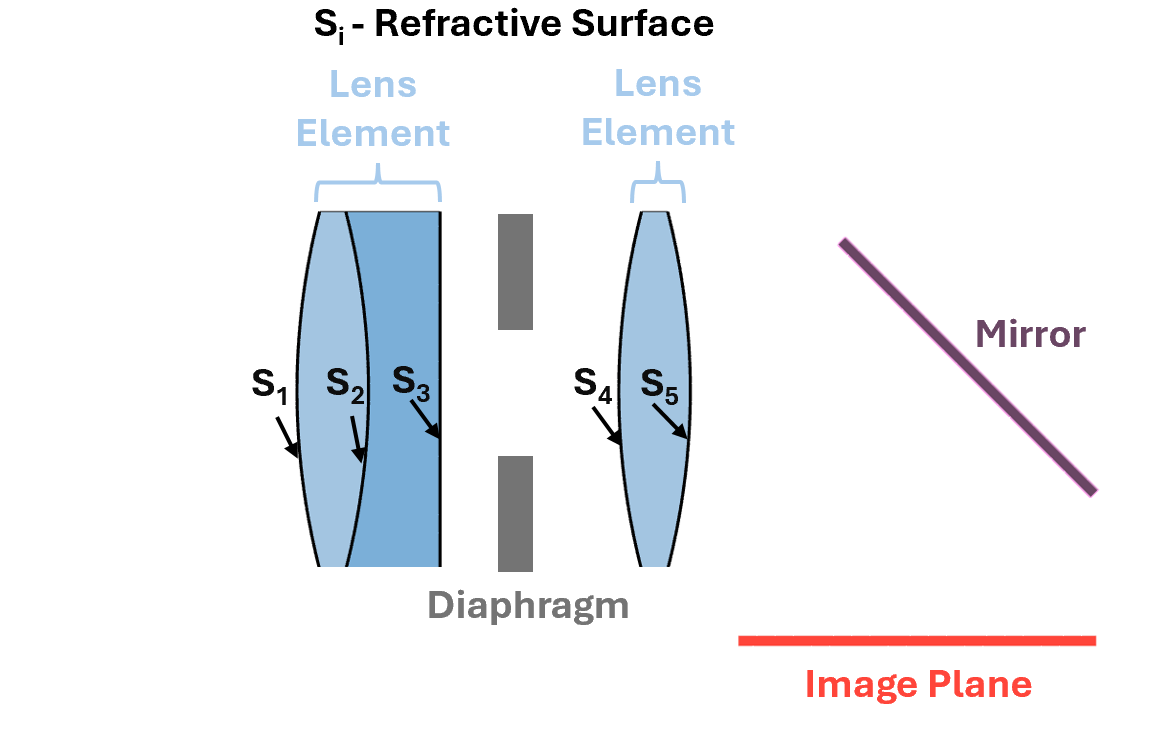
Add components to the system using these object functions.

• addRefractiveSurface — Create refractive surfaces which compose lens components. When you crate a lens element using this function, you create a LensElement object.

• addImagePlane — Create an image plane or sensor. When you create an image plane using this function, you create an ImagePlane object.

• addDiaphragm — Create a diaphragm or aperture stop. When you create an diaphragm using this function, you create a Diaphragm object.

• addMirror — Create a mirror. When you create a mirror component using this function, you create a Mirror object.

• addGap — Add a gap after a component or surface.

This image shows the types of components that you can add to an optical system using these object functions. Create lens elements by adding two or more refractive surfaces in sequence to an optical system.

For an example of how to create a lens system by adding components to an optical system, see Design Cooke Triplet.

Tip

You can use the setConstructionFrame object function to specify the position and angular orientation of the next components that you add. For example, you can use this function to tilt and position a mirror and the image plane. To learn more about optical coordinate systems, see Coordinate Systems in Optical Design.

Modify Optical Systems

To modify an existing optical system that you have imported or created, you can use these functions to insert, remove, or modify components and gaps:

• insert — Insert component before or after another component.

• remove — Remove a component.

• changeGap — Modify gap size of specified gap before or after the specified component.

• distanceAfter — Query the gap distance between a component and the subsequent component.

• distanceBefore — Query the gap distance between a component and the previous component.

Use Optical Materials

You can load optical materials for use in optical designs using a preloaded optical material library of vendor catalogs, or create your own custom optical materials. When you create an optical component such as a lens element or mirror, you can specify its optical material using the opticalMaterial object. To learn more about how to use optical materials, see Load, Create, and Use Optical Materials.

To create a UI that enables you to interactively visualize material properties of custom materials or materials from the library, use the opticalMaterialPicker.

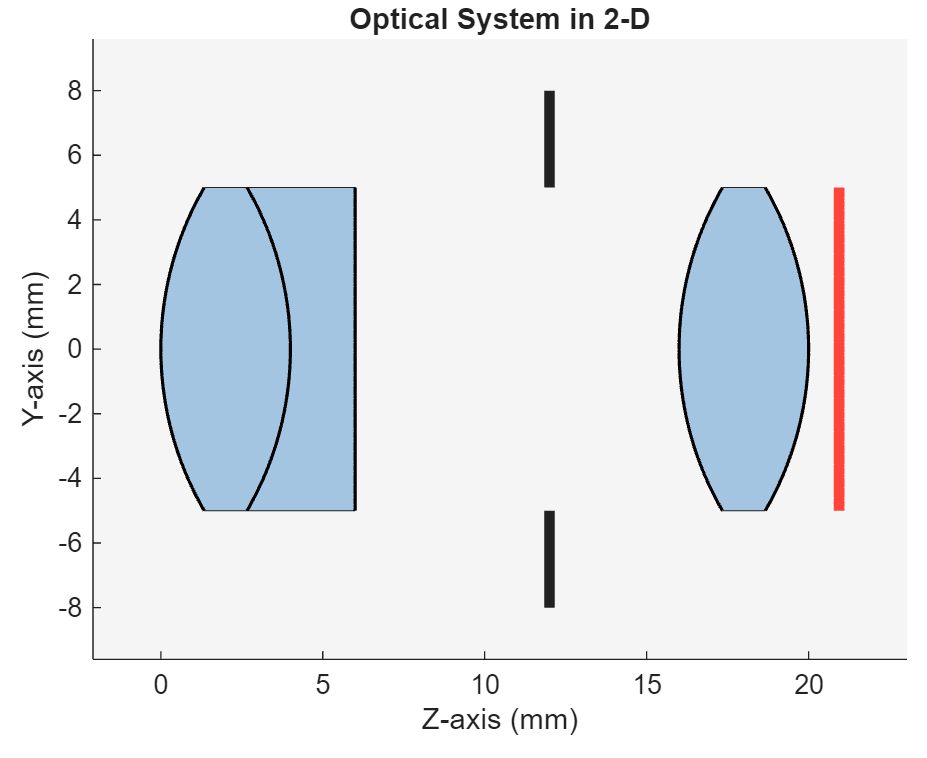
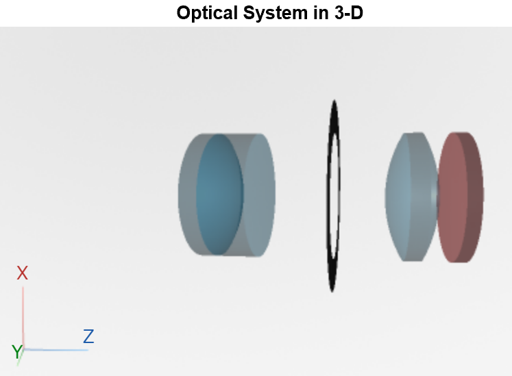
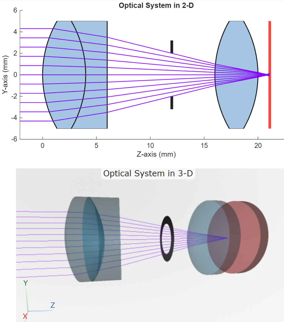
Visualize Optical Systems

Once you create an optical system, the view2d or view3d object function, respectively. The table visualizes the same optical system, containing a doublet lens, diaphragm, convex lens, and image plane, in 2-D and 3-D.

2-D Visualization	3-D Visualization
Visualize an optical system using the view2d function. view2d(opsys)	Visualize an optical system using the view3d function. view3d(opsys)

Apply Optical Coatings

Create an optical coating using the opticalCoating object, or select a default optical coating from the optical coating library using the pickCoating function. Apply the optical coating to all lens components in an optical system using the addCoating function, or assign an optical coating to the Coating property of LensElement or Mirror objects.

Use the fresnelCoefficients object function to perform reflectance, transmittance, and absorbance analysis for optical coating design with specific wavelength, light angle, and polarization requirements.

To get started with using optical coatings, see Apply Optical Coatings.

Perform Paraxial Analysis

Compute paraxial information to quickly evaluate the image quality and capabilities of your optical system before performing a full ray tracing analysis. Paraxial information of an optical system is the set of parameters that describe how the system behaves under the paraxial approximation, or the result of simplified ray tracing computations that assume small incoming ray angles relative to the optical axis. Paraxial quantities include cardinal points such as the system's focal and principal points, which are the fundamental reference points that define the paraxial imaging properties.

To compute paraxial information for an optical system, use the paraxialInfo object function. For an example of how to use paraxial information to optimize lens component positions in an optical system, see Optimize Photographic Zoom Lens Component Positions.

Configure Aperture, Focus, and Field of View

Prior to ray tracing analysis, you can tune your optical system by modifying the system aperture, focus, and field of view.

Modify System Aperture

The aperture of an optical system is the opening through which light enters the system. Its size controls the amount of light that reaches the image sensor or image plane. This image shows the effect of adding a diaphragm, a type of aperture stop, to an optical system that consists of a single convex lens and image plane. The addition of the diaphragm limits the system aperture and decreases the size of the blur spot formed on the image plane.

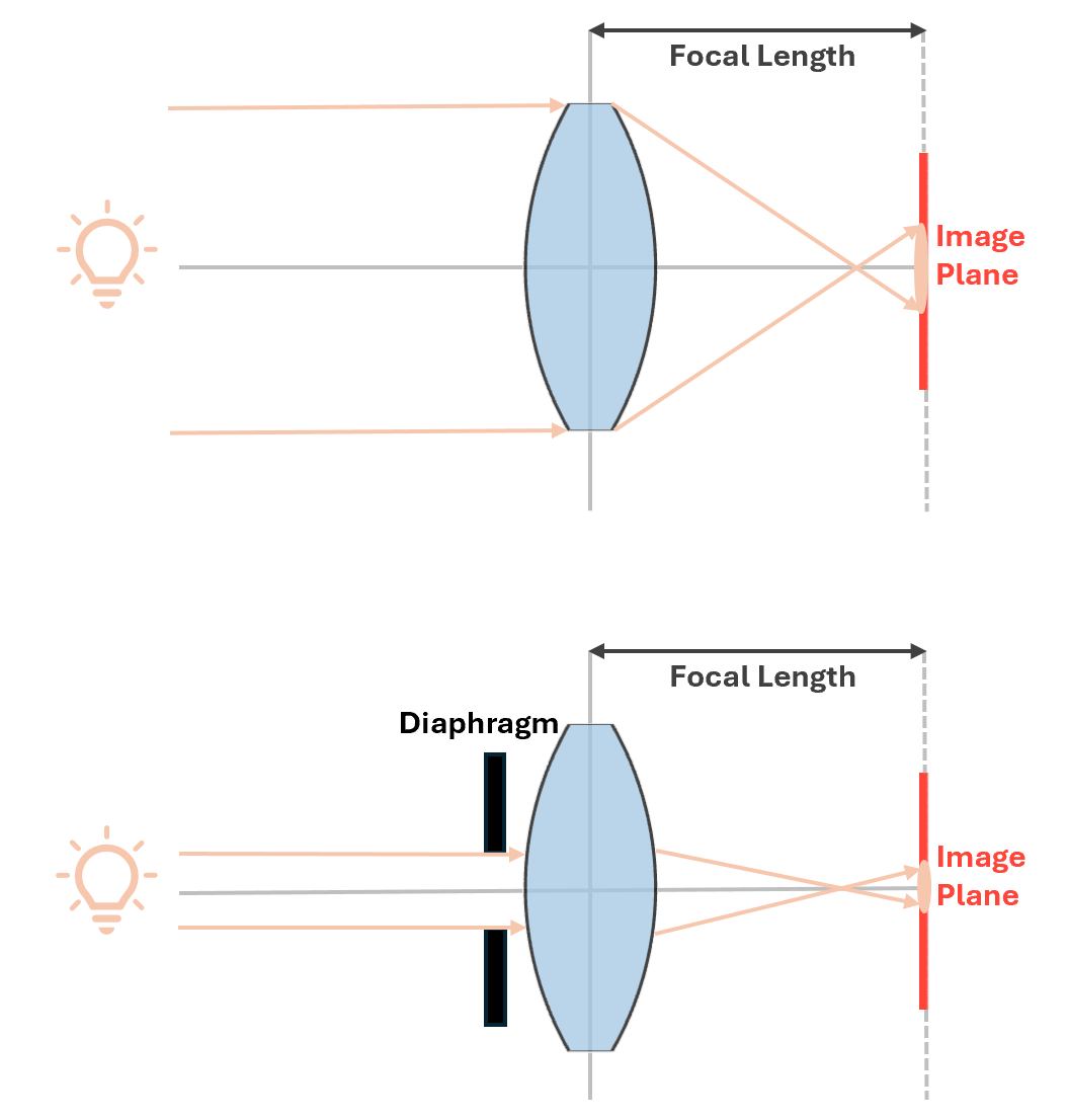
You can tune the size of the aperture of an optical system in these ways.

• Add Aperture Stop — Add a diaphragm to the optical system, which is an aperture stop that limits the cone of light entering the system. To add a diaphragm to an optical system, use the addDiaphragm object function.

• Resize Surface Semi-Diameters — Modify the semi-diameters of the optical system surfaces using the updateSemiDiameters object function. The semi-diameter of a surface is the circular aperture through which light passes, and is typically equal to half the diameter of the usable optical surface. Increase the semi-diameters of surfaces in the system to increase the system aperture size, allowing more light to enter the optical system.

Focus System and Tune Focal Length

To focus an optical system, minimize the spot size on the image plane by repositioning it. By moving the image plane, which often represents a sensor, you adjust the point at which light rays converge to form a clear image. To focus the optical system in this way, use the focus object function.

This image shows an unfocused optical system and the same system after it has been focused by repositioning the image plane.

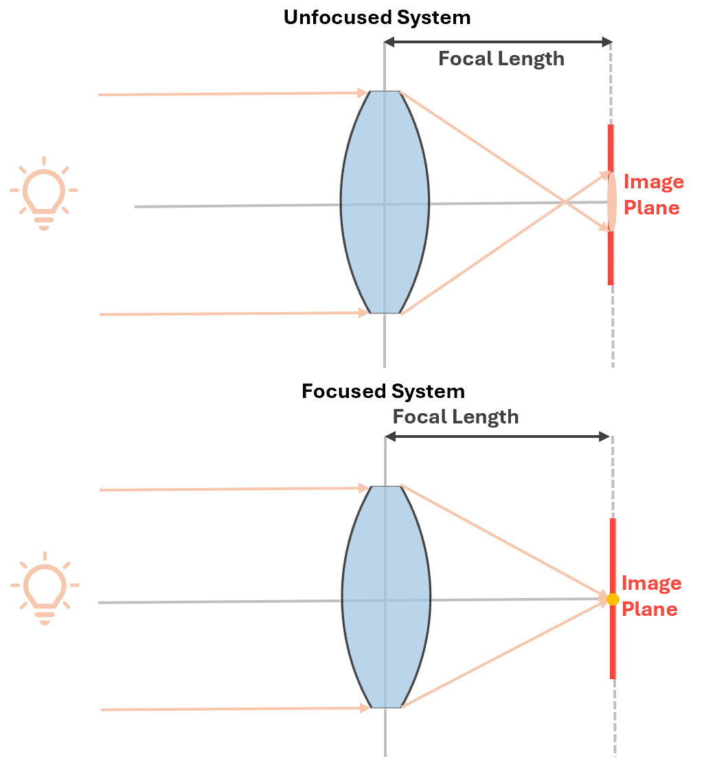
You can tune the focal length by adjusting the position of components. A shorter focal length brings the focus closer to the lens, while a longer focal length extends it further away. To learn how to tune optical component positions for a desired focal length, see these examples:

• Modify Focal Length By Scaling Optical System

• Optimize Photographic Zoom Lens Component Positions

Compute Half Field of View

For an imaging system, you can optionally tune the half field of view (HFOV) to set what part of the scene can be imaged. The HFOV is the maximum angle from the optical axis at which the system can accept a light ray from the edge of the field and focus it onto the image plane. The chief ray, the ray that passes through the center of the entrance pupil from an off-axis object point, defines the boundary of the field of view. This vertical field of view is the actual size of the area that is visible through the optical system. This diagram illustrates the HFOV and focal length of a simple optical system that consists of a single convex lens and an image plane.

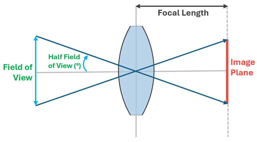
To compute the half field of view of an optical system, use the halfFieldOfView object function.

Tip

To limit vignetting, create an aperture to accommodate the light rays coming from the extremities of the HFOV. Vignetting is a reduction in image brightness or saturation at the periphery compared to the image center.

Perform Ray Tracing and Geometric Analysis

Using the Optical Design and Simulation Library for Image Processing Toolbox, you can create field points from which to trace rays, perform ray tracing, visualize spot diagrams, and perform aberration analysis of an optical system. To perform ray tracing and analysis, you must first add field points to the system.

Create Field Points

Create field points to represent the light source, or describe the object being imaged. You can create these types of field points.

• Field Angles: Field angles represent the angular position of a light source located at an infinite distance away from the first surface in the optical system. The chief ray, which passes through the center of the entrance pupil, defines the field angle.

• Field Positions: Field positions represent the actual spatial position of a light source, object point in the object plane, or the physical location of points on the imaged object.

To create field points, use the fieldPoint object function. To learn more, see Create Field Points.

Light emitted from field points first passes through the entrance pupil of the optical system. The entrance pupil is the effective aperture for incoming light, determining the angular cone of light that is accepted by the system. If the aperture stop is a lens surface, the entrance pupil is the effective aperture through which light travels. In this case, the aperture is shaped by the optical properties of the lens.

Perform Ray Tracing

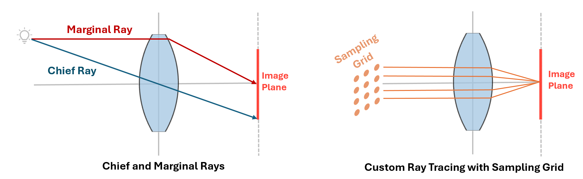
Perform ray tracing by simulating light ray paths as they travel from field points through the optical system. Ray tracing visualizations provide insight into how an optical system focuses light, the formation of images, and the presence of aberrations. You can trace these types of rays:

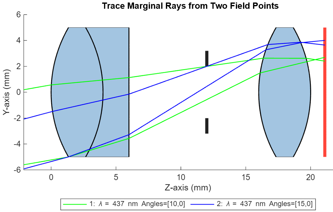
• Marginal rays: Marginal rays are outermost rays that pass through the edge of the system surfaces or aperture stop to the image plane.

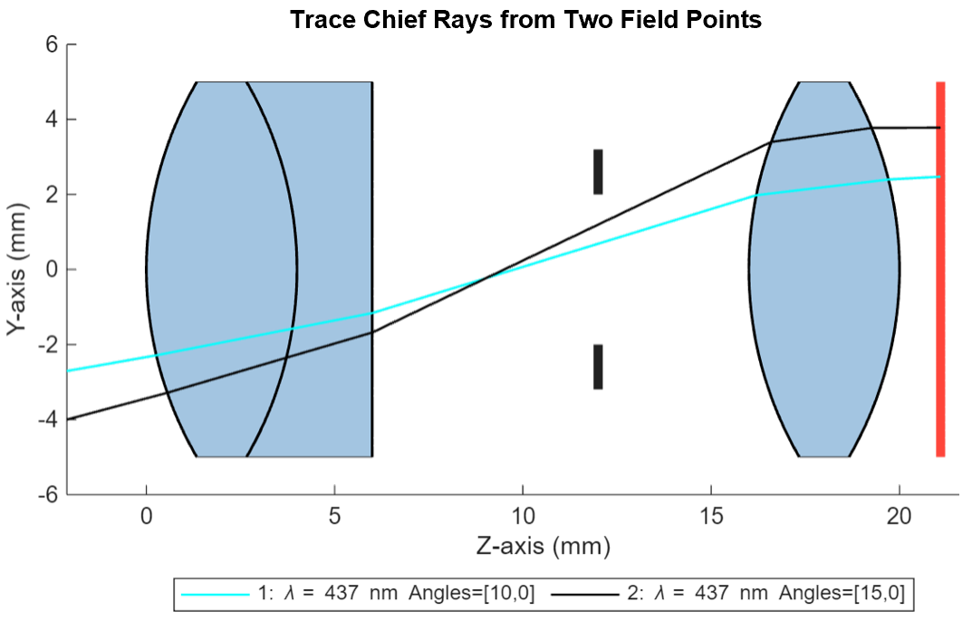
• Chief ray: The chief ray passes through the center of the entrance pupil halfway between the upper and lower marginal rays of the optical system.

• General rays: General rays are ray bundles that originate from field points and travel into the entrance pupil through the sampling grid. A sampling grid is an array of coordinate points defined in a plane perpendicular to the optical axis that defines the distribution of incoming light rays through the entrance pupil or another aperture of the system.

This image shows 2-D representations of an optical system. One illustrates tracing a chief ray and marginal ray originating from the same field point, and the other illustrates tracing a sampled group of general rays through the same system.

This table describes the ray tracing methods available in the library.

Ray Tracing Method	Implementation	Sample Visualization
Trace general rays through the system.	Trace rays using the traceRays object function. Optionally, specify a custom field point representation of the light source using the fieldPoint function. Optionally, specify the number of rays entering the system by creating a custom ray sampling grid using the samplingGrid function. Use the view2d or view3d object function to visualize the system in 2-D or 3-D, respectively. To add the ray representation to the visualization, use the addRays object function.
Trace marginal rays from each field point.	Trace marginal rays using the traceMarginalRays object function. Optionally, specify a custom field point representation of the light source using the fieldPoint function. Use the view2d or view3d object function to visualize the system in 2-D or 3-D, respectively. To add the ray representation to the visualization, use the addRays object function.
Trace a chief ray from each field point.	Trace a chief ray using the traceChiefRay object function. Optionally, specify a custom field point representation of the light source using the fieldPoint function. Use the view2d or view3d object function to visualize the system in 2-D or 3-D, respectively. To add the ray representation to the visualization, use the addRays object function.

To learn more about sampling traced rays, see Configure Ray Sampling in Optical System.

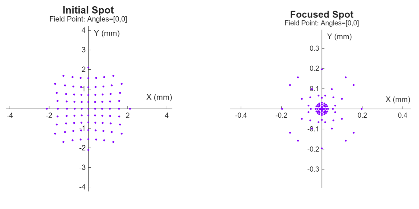
Visualize Spot Diagram

Spot diagrams provide a visual representation of how a system focuses light from a single field point. They illustrate the distribution of light rays at the image plane, revealing deviations from the ideal focus and highlighting aberrations such as astigmatism. The root mean square (RMS) spot size derived from these diagrams represents the average deviation of the rays from the centroid of the spot.

Compute the RMS spot size using the spot object function. Visualize the spot diagram in 2-D using the spotDiagram object function.

This image shows an example of a 2-D visualization of the spot diagrams for the optical system before and after the system has been focused. A smaller RMS spot size indicates higher optical quality and better focusing performance.

Analyze Image Quality

Analyze the aberrations, or deviations from the ideal image. This table describes the functions available for image quality analysis, and lists the objects which store their corresponding analysis results.

Function	Computed Aberration	Analysis Result Object
chromaticAberration	Chromatic aberration, or the discrepancy in focal length for different wavelengths, which causes color fringing and image blurring.	ChromaticAberration
fieldCurvature	Field curvature, or the curvature of the image plane, which leads to astigmatism and focus variations across the field of view.	FieldCurvature
rayAberration	Tangential and sagittal ray aberration, which leads to unequal focusing of light in different meridians and distorted or blurred images.	RayAberration
lensDistortion	Geometric lens distortion, or the deviation of light rays from their ideal paths.	LensDistortion

To visualize the result returned by each analysis function, use the show object function.

Compute Ray Path, Polarization, and Fresnel Coefficient Data

When you trace rays using the traceRays, traceMarginalRays, or traceChiefRays function, you can use the RayData property of the returned RayBundle object to inspect geometric information about each ray’s path through the optical system. Use this data to analyze key aspects of ray geometry, such as origins, intersection points, directions, and how rays terminate.

Additionally, you can use the RayProperties name-value argument of the ray tracing functions to return this additional ray data:

• Surface normal vectors at intersections

• Angle of incidence at each surface

• Cumulative optical path length (OPL)

• Intersection points in local surface coordinates

Using the RayProperties name-value argument of the traceRays function, you can additionally return this data for polarization analysis:

• Polarization transformation matrices (bulk, surface, system)

• Fresnel reflection/transmission coefficients, power coefficients, bulk transmission and phase shift, total system transmittance

References

[1] Bass, Michael, editor-in-chief. Handbook of Optics, Volume 2. 2nd ed. Edited by Eric W. Van Stryland, David R. Williams, and William L. Wolfe. New York: McGraw-Hill, 1995.