Optimize Photographic Zoom Lens Component Positions

This example uses:

Optical Design and Simulation Library for Image Processing Toolbox Optical Design and Simulation Library for Image Processing Toolbox
Optimization Toolbox Optimization Toolbox

This example demonstrates how to use numerical optimization techniques to optimize the positions of zoom groups and achieve a target focal length. A zoom group is a series of optical elements that have fixed positions relative to each other. Photographic zoom lenses are lenses that have a variable focal length, enabling photographers to zoom in or out on a subject without switching to a different lens. These lenses can contain multiple zoom groups that can be moved to change the focal length of a system.

In this example, you optimize zoom group positions to obtain a target focal length and RMS spot size. The RMS spot size quantifies how closely to the focal point the light rays converge at the image plane, which is crucial for determining the sharpness and clarity of the image produced by the optical system.

This example requires the Optical Design and Simulation Library for Image Processing Toolbox™ and the Optimization Toolbox™. You can install the Optical Design and Simulation Library for Image Processing Toolbox from Add-On Explorer. For more information about installing add-ons, see Get and Manage Add-Ons.

Visualize Moveable Zoom Component Groups

The reference optical system design is a 70–210 mm F/2.8–4 zoom lens with two moveable zoom groups [1]. This system contains these distinct parts:

The focus group containing components C1 and C2 (fixed).
The first zoom group containing the two doublets, C3 and C4 (moveable).
The second moveable zoom group containing the components from C5 to C12 (moveable).
The image plane C13, at a fixed location (fixed).

The relative positions of the components within each of the two moveable groups is fixed.

Load Photographic Zoom System Configurations

Load two photographic zoom optical systems, opsysz1 and opsysz2, with different positionings of the two moveable component groups using the createPhotoZoom helper function. The function is attached to this example as a supporting file.

opsysz1 = createPhotoZoom(ZoomPosition=1);
opsysz2 = createPhotoZoom(ZoomPosition=2);

Compute Focal Length

To compute the focal length of each system, compute the paraxial information for each optical system using the paraxialInfo object function.

paraxialz1 = paraxialInfo(opsysz1);
paraxialz2 = paraxialInfo(opsysz2);

Define the focal length of each optical system using the FocalLength property of the corresponding ParaxialInfo object.

fz1 = paraxialz1.FocalLength

fz1 = 
72.0158

fz2 = paraxialz2.FocalLength

fz2 = 
203.7305

Visualize Moveable Component Groups

Trace the marginal rays through each optical system using the traceMarginalRays object function.

raysz1 = traceMarginalRays(opsysz1);
raysz2 = traceMarginalRays(opsysz2);

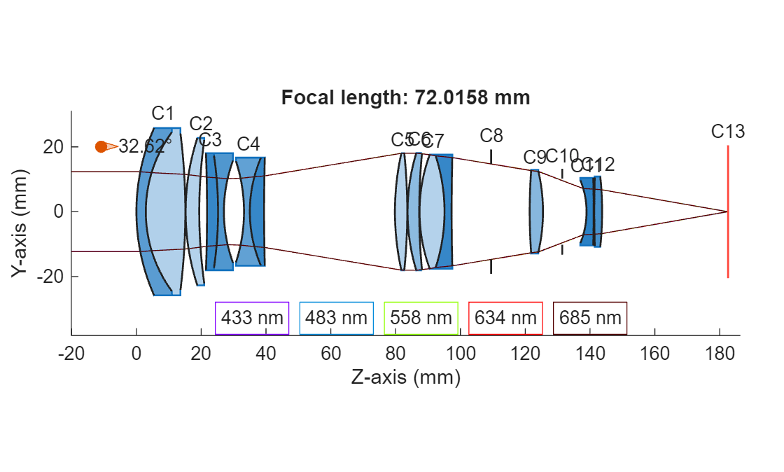
Display a 2-D visualization of the optical system in the first configuration using the view2d function, and visualize the traced marginal rays through the system using the addRays object function.

hv = view2d(opsysz1,Title="Focal length: "+fz1+" mm",Labels="component");
addRays(hv,raysz1)

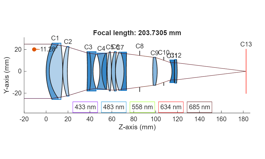
Display a 2-D visualization of the optical system in the second configuration, and visualize the traced marginal rays through the system. Note that the focal length is larger in the second scenario due to differences in the gap between components C2 and C3 and the gap between components C4 and C5.

hv = view2d(opsysz2,Title="Focal length: "+fz2+" mm",Labels="component");
addRays(hv,raysz2)

Determine Component Position Ranges

Model the possible configuration of the two moveable zoom groups using the two previously established variables: the gap between C2 and C3 and the gap between C4 and C5. To ensure that each configuration results in a physical system without component overlap, you must determine the maximum value of the sum of the two gaps.

Load a photographic zoom lens optical system using the createPhotoZoom helper function, and display a 2-D visualization of the system.

opsys = createPhotoZoom;
view2d(opsys,Labels="surface");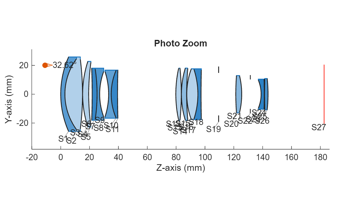

The first focus group and the last component, the image plane, must remain fixed. Thus, the space where both zoom groups can exist is between the second surface of component C2 (surface S5) and the first surface of component C13 (surface S27).

Define Range of Moveable Components

Define the global positions of all surfaces in the system using the SurfaceTable property of the opticalSystem object opsys. Define the surface positions using only the *z-*coordinate, as the optical system is fully aligned with the z-axis.

stbl = opsys.SurfaceTable;
surfacePositions = stbl.Position(:,3);

Compute the distance between the first focus group and the image plane, which typically contains a sensor.

d_5_Sensor = surfacePositions(27) - surfacePositions(5);

Compute the thickness of the first zoom component.

d_6_11 = surfacePositions(11) - surfacePositions(6);

Compute the thickness of the second zoom component.

d_12_26 = surfacePositions(26) - surfacePositions(12);

Compute the maximum physical value of the sum of the two gaps between components (from C2 to C3 and from C4 to C5). This is the maximum value either of two distances, C2 to C3 or C4 to C5, can take when the other is 0. You can use this value as a constraint when optimizing component positions.

dMax = d_5_Sensor - d_6_11 - d_12_26;

Minimize Merit Function

Use the merit function to achieve a specified focal length and satisfy additional optical constraints, such as an optimal RMS spot size. The merit function must return a scalar value that quantifies the deviation of the proposed solution from the target value. The optimizer then aims to minimize this deviation. In this section, you minimize the merit function and optimize the zoom group positions by using the fmincon (Optimization Toolbox) function.

Load an optical system with moveable zoom groups.

opsys = createPhotoZoom;

Save the position of the image plane, which must remain fixed, to the UserData property.

opsys.UserData.FixedImagePlanePosition = surfacePositions(27);

Define a set of focal lengths for which to optimize zoom group positions.

targetFocalLengths = 70:5:210;

Initialize a matrix for containing the solutions returned by the fmincon function.

zoomGrpDistances = zeros(numel(targetFocalLengths),2);

Define a sample solution for the optimizer to test of the form [gap1 gap2], where gap1 is the gap between C2 and C3, and gap2 is the gap between C4 and C5.

distSol = [distanceAfter(opsys,2) distanceAfter(opsys,4)];

Determine solutions for each focal length independently. Construct the merit function using the opticalMeritFunc, helper function and specify it to the fmincon function as the objective function to minimize. If you have a Parallel Computing Toolbox™, compute the solutions in parallel.

parfor ind = 1:numel(targetFocalLengths)
    problem = struct;
    problem.x0 = distSol;
    % Express the total distance constraint, A.x <= b. The sum of the two
    % distances must be less than or equal to dMax.
    problem.A = [1 1];
    problem.b = dMax;

    % Set a lower bound to prevent first zoom group from intersecting the
    % focus group. This constraint can also come from mechanical
    % limitations in the manufacturing processing.
    problem.lb = [1 0];

    % Specify solver and solver options.
    problem.solver = "fmincon";
    problem.options = optimoptions("fmincon");
    problem.options.Display = "none";
    % Optionally, display more information by uncommenting the next line.
    %problem.options.Display ="iter-detailed";

    % The current merit function is insensitive to the default step size.
    % Increase the step size to ensure the merit functions changes for
    % small deltas in the candidate solutions.
    problem.options.FiniteDifferenceStepSize = 1e-3;

    % Increase step tolerance to improve runtime efficiency. You can reduce
    % the step tolerance to potentially get better results at the cost of 
    % additional runtime.
    problem.options.StepTolerance = 1e-2;

    % Set the optical merit function, using the opticalMeritFunc helper 
    % function as the objective function for the optimizer.
    problem.objective = @(x)opticalMeritFunc(x,opsys,targetFocalLengths(ind));

    % Run the optimizer using the fmincon function.
    [zoomGrpDistances(ind,:),fval,exitflag,output] = fmincon(problem);
end

Starting parallel pool (parpool) using the 'Processes' profile ...
09-Jan-2026 18:16:26: Job Queued. Waiting for parallel pool job with ID 3 to start ...
Connected to parallel pool with 4 workers.

Visualize Optimization Results

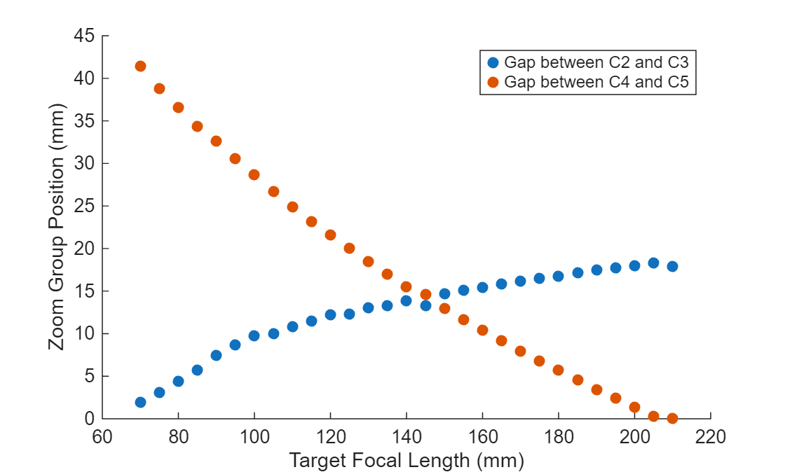
Plot the solutions, the optimized zoom group positions, as a function of the corresponding target focal lengths.

figure
scatter(targetFocalLengths,zoomGrpDistances,"filled")
xlabel("Target Focal Length (mm)")
ylabel("Zoom Group Position (mm)")
legend("Gap between C2 and C3","Gap between C4 and C5")

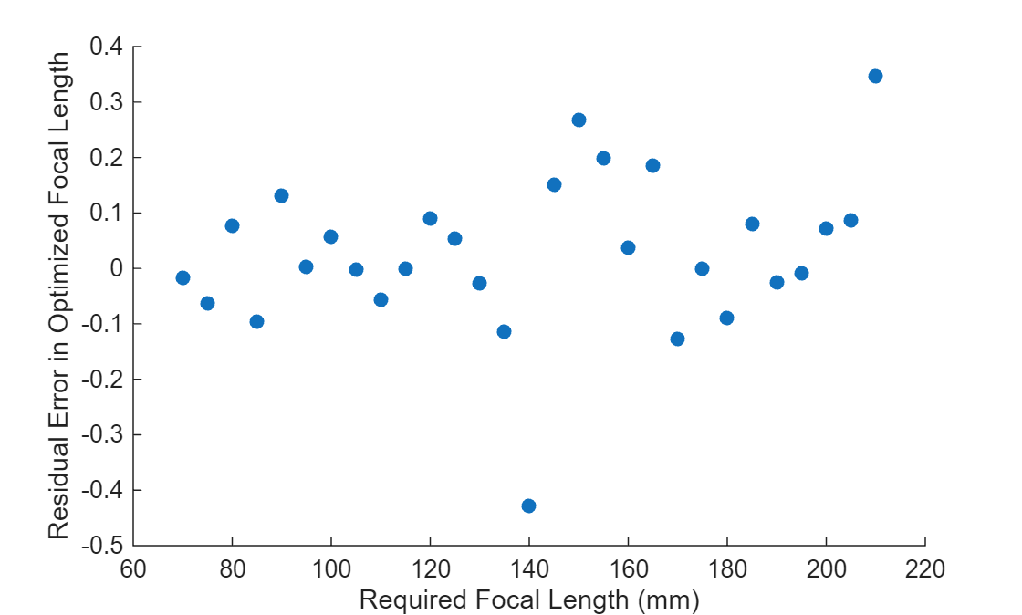
Inspect Residual Error

Compute the residual error, the difference between the target focal length and the optimized focal length, for each target focal length optimization.

optimFocalLengths = zeros(size(targetFocalLengths));
for ind = 1:numel(targetFocalLengths)
    % Compute the focal length as a result of optimization.
    opsys = configureForOptimization(opsys,zoomGrpDistances(ind,:));
    opsysParInfo = paraxialInfo(opsys);
    optimFocalLengths(ind) = opsysParInfo.FocalLength;
end
residualError = targetFocalLengths - optimFocalLengths;

Plot the residual error.

figure
scatter(targetFocalLengths,residualError,"filled")
xlabel("Required Focal Length (mm)")
ylabel("Residual Error in Optimized Focal Length")

Analyze Optimized System

Specify an initial zoom level at which to optimize the zoom group component position. Optimize the system using the configureForOptimization helper function.

Create a tiled figure in which to plot the results. Display a 2-D visualization of the optimized optical system using the view2d object function, and visualize the traced marginal rays through the system. Visualize the spot diagram and the chromatic aberration using the show object function. Specify a zoom level at which to modify the zoom group component position and trace rays, and compute the RMS spot size and chromatic aberration.

zoomLevel = 15;
distSol = zoomGrpDistances(zoomLevel,:);
opsys = configureForOptimization(opsys,distSol);
tl = tiledlayout(2,2);
nexttile([1 2])
hv = view2d(opsys,Parent=tl);
hv.Title = "Focal length:" + paraxialInfo(opsys).FocalLength;
rays = traceMarginalRays(opsys,Wavelengths=opsys.PrimaryWavelength);
addRays(hv,rays)

nexttile
show(spot(opsys),Parent=tl);

nexttile
show(chromaticAberration(opsys),Parent=tl);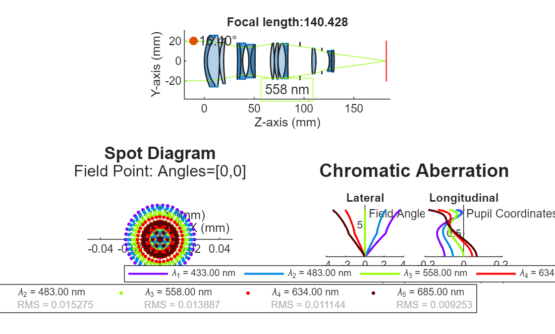

Helper Functions

`configureForOptimization`

To evaluate a candidate solution, the configureForOptimization helper function updates the gaps between each of the two zoom groups based on the solution value.

function opsys = configureForOptimization(opsys,sampleSolution)
% Change the gap between each of the two component groups.
changeGap(opsys,2,sampleSolution(1),GapLocation="after");
changeGap(opsys,4,sampleSolution(2),GapLocation="after");
% Since all components after the second component are modified, 
% keep the image plane fixed at its initial position.
opsys.Components(end).Position(3) = opsys.UserData.FixedImagePlanePosition;
end

`opticalMeritFunc`

The opticalMeritFunc helper function takes as inputs the optimizer's current proposed distance solution, an opticalSystem object containing the optical system to optimize, and the target focal length. To quantify the accuracy of the solution, it returns a system error value that is the sum of the absolute deviation of the actual focal length and RMS spot values from the target values.

Due to the relative size differences in the target focal length and RMS spot size, the focal length error term dominates the system error. To scale the focal length and spot size error to the same order of magnitude, multiply each error term by the corresponding weights fWeight and sWeight. To use this helper function for your application, adjust the weight terms appropriately to ensure that each component error contribution to the system error is of the same order of magnitude.

function errorTerm = opticalMeritFunc(x,opsys,targetFocalLength)
% Load a sample configuration tested by the optimizer.
opsys = configureForOptimization(opsys,x);
% Evaluate how much this configuration deviates from required values
% by computing the system error, or the deviation from target.
try
    % Compute the focal length and spot size of a candidate system
    % that the optimizer function is evaluating.
    zParaxial = paraxialInfo(opsys);
    % Compute the focal length. 
    actualFocalLength = zParaxial.FocalLength;
    % Compute the spot size.
    spotRes = spot(opsys,Wavelength=opsys.PrimaryWavelength);
    % Specify a target small target RMS spot size, in millimeters.
    targetSpotSize = 0.01;
    % Introduce weight terms to scale both focal length and spot size
    % to the same order of magnitude. 
    fWeight = 1;
    sWeight = 10;
    %Compute the error term.
    errorTerm = fWeight*abs(targetFocalLength - actualFocalLength) + ...
        sWeight*abs(spotRes.RMS - targetSpotSize);
catch
    % If an error occurs when evaluating a solution, return inf to
    % indicate a poor solution.
    errorTerm = inf;
end
end

References

[1] Bass, Michael and Optical Society of America, eds. "Chapter 16: Camera Lenses". Handbook of Optics. 2nd ed. Vol. II. New York: McGraw-Hill, 1995. pp 16.20-16.21.