このページは機械翻訳を使用して翻訳されました。最新版の英語を参照するには、ここをクリックします。
Simulink モデルを並列に最適化
この例では、複数の Global Optimization Toolbox ソルバーを使用して Simulink ® モデルを並列に最適化する方法を示します。この例では、内部的に parsim を呼び出して並列計算を実行するベクトル化された計算を使用します。
モデルと目的関数
ローレンツ方程式は連立常微分方程式です (ローレンツ方程式を参照)。実定数およびの場合、このシステムは
高感度システムのパラメーターのローレンツ値は と です。方程式を [x(0),y(0),z(0)] = [10,20,10] から始め、時間 0 から 100 までの方程式の変化を表示します。
sigma = 10;
beta = 8/3;
rho = 28;
f = @(t,a) [-sigma*a(1) + sigma*a(2); rho*a(1) - a(2) - a(1)*a(3); -beta*a(3) + a(1)*a(2)];
xt0 = [10,20,10];
[tspan,a] = ode45(f,[0 100],xt0);     % Runge-Kutta 4th/5th order ODE solver
figure
plot3(a(:,1),a(:,2),a(:,3))
view([-10.0 -2.0])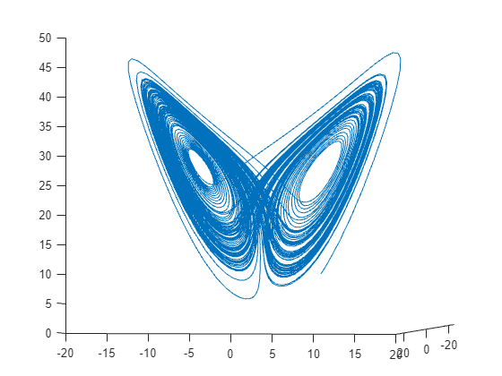
変化はかなり複雑です。しかし、短い時間間隔では、このシステムはある程度等速円運動のように見えます。時間間隔 [0,1/10] にわたり、解をプロットします。
[tspan,a] = ode45(f,[0 1/10],xt0);     % Runge-Kutta 4th/5th order ODE solver
figure
plot3(a(:,1),a(:,2),a(:,3))
view([-30 -70])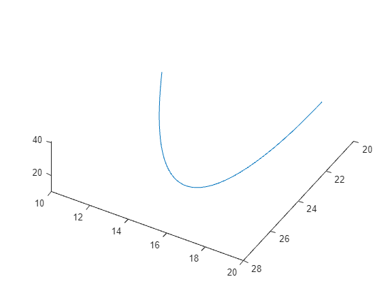
等速円運動はいくつかのパラメーターに依存します。
x-y平面からのパスの角度
x軸に沿った傾斜からの平面の角度
速度
半径
時間オフセット
3Dオフセット
これらのパラメーターを等速円運動に関連付け、ローレンツ システムに適合させる詳細については、例 常微分方程式 (ODE) の適合 を参照してください。
目的関数は、0 から 1/10 までの一連の時間にわたって、ローレンツ システムと等速円運動の差の二乗和を最小化することです。xdata倍の場合、目的関数は
objective = sum((fitlorenzfn(x,xdata) - lorenz(xdata)).^2) - (F(1) + F(end))/2
ここで、fitlorenzfn は等速円運動の経路上の点を計算し、lorenz(xdata) は時刻 xdata におけるローレンツ システムの 3D 進化を表し、F は円運動とローレンツ システムの対応する点間の距離の 2 乗のベクトルを表します。目的は、エンドポイントの値の半分を減算して、積分を最もよく近似することです。
一致する曲線として等速円運動を考慮し、シミュレーション内のローレンツパラメーターを変更して目的関数を最小化します。
Simulink モデル
この例を実行すると使用できる Lorenz_system.slx ファイルは、Lorenz システムを実装します。
等速円運動のデータを入力します。
x = zeros(8,1);
x(1) = 1.2814;
x(2) = -1.4930;
x(3) = 24.9763;
x(4) = 14.1870;
x(5) = 0.0545;
x(6:8) = [13.8061;1.5475;25.3616];
Lorenz システムをロードし、基本パラメーターを使用してシミュレートします。結果として得られるシステムの 3D プロットを作成し、等速円運動と比較します。
model = "Lorenz_system";
open_system(model);
Warning: Unrecognized function or variable 'CloneDetectionUI.internal.CloneDetectionPerspective.register'.
in = Simulink.SimulationInput(model);
% params [X0,Y0,Z0,Sigma,Beta,Rho]
params = [10,20,10, 10,8/3,28]; % The original parameters Sigma, Beta, Rho
in = setparams(in,model,params);
out = sim(in);

yout = out.yout;
h = figure;
plot3(yout{1}.Values.Data,yout{2}.Values.Data,yout{3}.Values.Data,"gx");
view([-30 -70])

tlist = yout{1}.Values.Time;
YDATA = fitlorenzfn(x,tlist);
hold on
plot3(YDATA(:,1),YDATA(:,2),YDATA(:,3),"kx")
hold off
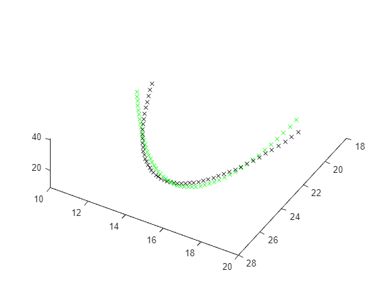
プロットされた時間の曲線間の差の二乗和を計算します。
ssq = objfun(in,params,YDATA,model)
ssq =
26.9975
Simulink モデルパラメーターを並列に最適化
ソルバーが並列計算を行う仕組み で説明されているように、Global Optimization Toolbox ソルバーは通常、内部で parfor または parfeval を呼び出して並列計算を行います。ただし、Simulink モデルは並列計算でこれらの関数をサポートしていません。
Simulink モデルを並列に最適化するには、次のような目的関数を記述します。
入力として行列を受け入れます。行列の各行はパラメーターのベクトルです。
parsimを呼び出して並列シミュレーションを実行します値のベクトルを返します。ベクトルの各エントリには、入力行列の1行のパラメーターに対応する目的関数の値が含まれます。
目的関数が入力として行列を受け入れるようにするには、ソルバー UseVectorized オプションを true に設定します。UseParallel オプションを true に設定しないでください。目的関数は、パラメーターベクトルを Simulink 変数にマッピングし、Simulink 結果をパラメーターにマッピングする必要があります。
次に示す parobjfun ヘルパー関数はパラメーターの行列を受け入れます。行列の各行は 1 セットのパラメーターを表します。この関数は、setparams ヘルパー関数 (この例の最後に表示) を呼び出して、Simulink.SimulationInput ベクトルのパラメーターを設定します。次に、parobjfun 関数は parsim (Simulink) を呼び出して、パラメーターに基づいてモデルを並列に評価します。
function f = parobjfun(params,YDATA,model)
% Solvers can pass different numbers of points to evaluate.
% N is the number of points on which the simulation must be performed.
N = size(params,1);

% Create a vector of size N simulation inputs for the model.
simIn(1:N) = Simulink.SimulationInput(model);

% Initialize the output.
f = zeros(N,1);

% Map the optimization parameters (params) to each SimulationInput.
for i = 1:N
    simIn(i) = setparams(simIn(i),model,params(i,:));
end

% Set the parsim properties and perform the simulation in parallel.
simOut = parsim(simIn,ShowProgress="off", ...
    UseFastRestart="on");

% Fetch the simulation outputs (a blocking call) and compute the final outputs.
for i = 1:N
    yout = simOut(i).yout;
    vals = [yout{1}.Values.Data,yout{2}.Values.Data,yout{3}.Values.Data];
    g = sum((YDATA - vals).^2,2);
    f(i) = sum(g) - (g(1) + g(end))/2;
end
end
等速円運動に合わせる準備をする
まだ開いていない場合は並列プールを開きます。並列オプションの設定に応じて、プールは自動的に開くことができます。最初の並列ソルバーの実行中に並列プールを開く時間をカウントしないようにするには、ここで並列プールを開きます。
pool = gcp("nocreate"); % Check whether a parallel pool exists.
if isempty(pool) % If not, create one.
    pool = parpool;
end
ソルバーの境界を現在のパラメーター値の 20% 上と下に設定します。
lb = 0.8*params;
ub = 1.2*params;
速度を上げるには、シミュレーションで高速再起動を使用するように設定します。
set_param(model,FastRestart="on");
c = onCleanup(@()closeModel(model));
再現性のためにランダムストリームを設定します。
rng(1)
目的関数を、追加のパラメーターを持つ parobjfun として定義します。
fitobjective = @(params)parobjfun(params,YDATA,model);
ソルバー間の公平な比較を行うには、ソルバーごとに関数評価の最大数を約 300 に設定します。
maxf = 300;
patternsearch "nups" アルゴリズム
patternsearch "nups" アルゴリズムのオプションを設定します。UseVectorized を true に設定し、psplotbestf および psplotmeshsize プロット関数を使用するようにオプションを設定します。
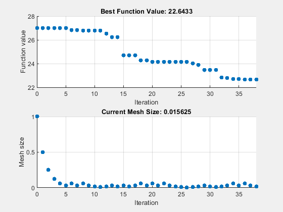
options = optimoptions("patternsearch",...
    UseVectorized=true,Algorithm="nups",...
    MaxFunctionEvaluations=maxf,PlotFcn={"psplotbestf" "psplotmeshsize"});
ソルバーを呼び出して、二乗和とシミュレーション時間の改善を表示します。
rng(1)
tic
[fittedparamspsn,fvalpsn] = patternsearch(fitobjective,params,[],[],[],[],lb,ub,[],options);
patternsearch stopped because it exceeded options.MaxFunctionEvaluations.
paralleltimepsn = toc
paralleltimepsn =
221.8100
disp([ssq,fvalpsn])
26.9975 22.6433
patternsearch "classic" アルゴリズム
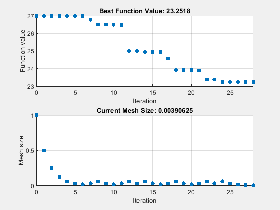
patternsearch "classic" アルゴリズムのオプションを設定します。UseVectorized を true に設定し、psplotbestf および psplotmeshsize プロット関数を使用するようにオプションを設定します。"classic" アルゴリズムでベクトル化を使用するには、UseCompletePoll オプションを true にも設定する必要があります。
options = optimoptions("patternsearch",...
    UseVectorized=true,UseCompletePoll=true, ...
    Algorithm="classic",...
    MaxFunctionEvaluations=maxf,PlotFcn={"psplotbestf" "psplotmeshsize"});
tic
[fittedparamspsc,fvalpsc] = patternsearch(fitobjective,params,[],[],[],[],lb,ub,[],options);
patternsearch stopped because it exceeded options.MaxFunctionEvaluations.

paralleltimepsc = toc
paralleltimepsc =
147.6369
disp([ssq,fvalpsc])
26.9975 23.2518
遺伝的アルゴリズム
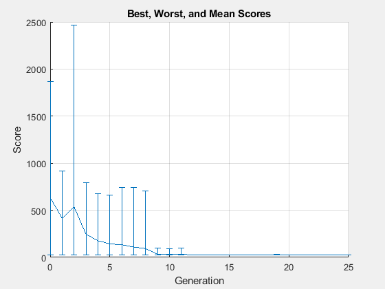
遺伝的アルゴリズムのオプションを設定します。ga の母集団サイズを、最適化されるパラメーターの数の 2 倍に設定します。開始点 params を初期母集団として渡すと、この比較的良好な点が初期母集団の一部になります。ga で約 maxf 個の個体を評価するには、最大世代数を maxf/母集団サイズに設定します。UseVectorized を true に設定します。
rng(1)
PopSize = 2*numel(params);
options = optimoptions("ga",PopulationSize=PopSize,...
    UseVectorized=true,InitialPopulationMatrix=params,...
    MaxGenerations=round(maxf/PopSize),PlotFcn="gaplotrange");
tic
[fittedparamsga,fvalga] = ga(fitobjective,numel(params),[],[],[],[],lb,ub,[],options);
ga stopped because it exceeded options.MaxGenerations.
paralleltimega = toc
paralleltimega =
152.9136
disp([ssq,fvalga])
26.9975 24.8405
サロゲート最適化
サロゲート最適化のオプションを設定します。BatchSize オプションを、最適化されるパラメーターの数の 2 倍に設定します。関数評価の最大数を、maxf を超えないバッチ サイズの最大倍数に設定します。UseVectorized を true に設定します。
rng(1)
BatchSize = 2*numel(params);
myn = floor(maxf/BatchSize)*BatchSize; % Multiple of BatchSize
options = optimoptions("surrogateopt",BatchUpdateInterval=BatchSize,...
    UseVectorized=true,InitialPoints=params,...
    MaxFunctionEvaluations=myn,PlotFcn="optimplotfvalconstr");
tic
[fittedparamssurr,fvalsurr] = surrogateopt(fitobjective,lb,ub,[],[],[],[],[],options);
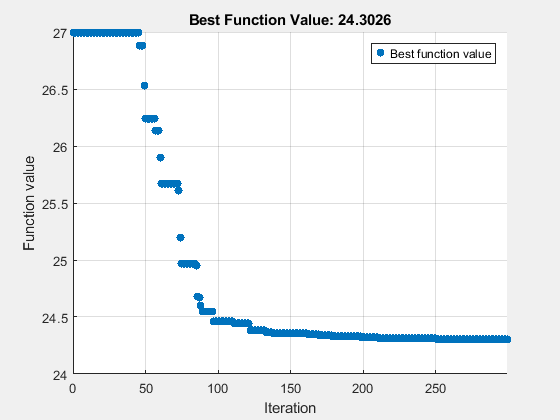
surrogateopt stopped because it exceeded the function evaluation limit set by
'options.MaxFunctionEvaluations'.
paralleltimesur = toc
paralleltimesur =
209.8845
disp([ssq,fvalsurr])
26.9975 24.3026
粒子群最適化
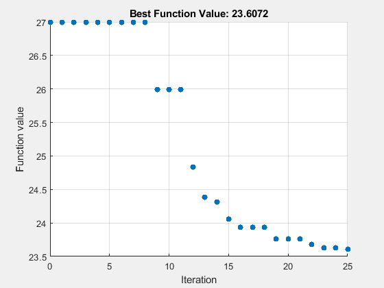
粒子群最適化のオプションを設定します。群れのサイズを、最適化されるパラメーターの数の 2 倍に設定します。反復の最大回数を maxf/swarm サイズに設定します。UseVectorized を true に設定します。
rng(1)
options = optimoptions("particleswarm",SwarmSize=PopSize,...
    MaxIterations=round(maxf/PopSize),InitialPoints=params,...
    UseVectorized=true,PlotFcn="pswplotbestf");
tic
[fittedparamspsw,fvalpsw] = particleswarm(fitobjective,numel(params),lb,ub,options)
Optimization ended: number of iterations exceeded OPTIONS.MaxIterations.
fittedparamspsw = 1×6

   10.4450   19.8899    9.8416    9.4086    2.6612   27.8898
fvalpsw =
23.6072
paralleltimepsw = toc
paralleltimepsw =
274.8291
disp([ssq,fvalpsw])
26.9975 23.6072
非並列計算と比較
比較のために、UseVectorized オプションを false に設定して、patternsearch "classic" アルゴリズムをシリアルで実行します。
options = optimoptions("patternsearch",...
    UseVectorized=false,UseCompletePoll=true, ...
    Algorithm="classic",...
    MaxFunctionEvaluations=maxf,PlotFcn={"psplotbestf" "psplotmeshsize"});
tic
[fittedparamspscs,fvalpscs] = patternsearch(fitobjective,params,[],[],[],[],lb,ub,[],options);
patternsearch stopped because it exceeded options.MaxFunctionEvaluations.
serialltimepscs = toc
serialltimepscs =
1.4635e+03
disp([ssq,fvalpscs])
26.9975 23.2518
非ベクトル化 (シリアル) 最適化はベクトル化 (並列) 最適化よりもはるかに長い時間がかかり、並列 patternsearch "classic" アルゴリズムと同じソリューションに到達します。
結果を要約する
各ソルバーのタイミングと最適な関数値に関する結果を収集します。
table(["NUPS";"PSClassic";"ga";"surr";"particleswarm";"PSClassicSerial"],...
    [paralleltimepsn;paralleltimepsc;paralleltimega;paralleltimesur;paralleltimepsw;serialltimepscs], ...
    [fvalpsn;fvalpsc;fvalga;fvalsurr;fvalpsw;fvalpscs],...
    'VariableNames',{'Algorithm' 'Time' 'FVal'})
ans=6×3 table
        Algorithm         Time      FVal
    _________________    ______    ______

    "NUPS"               221.81    22.643
    "PSClassic"          147.64    23.252
    "ga"                 152.91     24.84
    "surr"               209.88    24.303
    "particleswarm"      274.83    23.607
    "PSClassicSerial"    1463.5    23.252
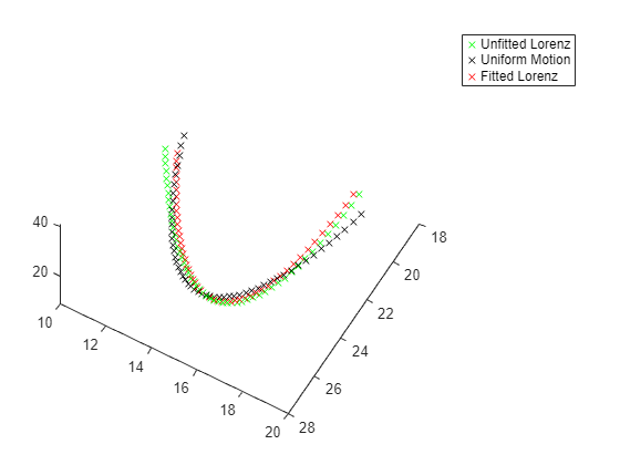
patternsearch "nups" アルゴリズムは目的関数の値が最も低くなります。そのアルゴリズムの結果の軌跡をプロットします。
figure(h)
hold on
in = setparams(in,model,fittedparamspsn);
out = sim(in);
yout = out.yout;
plot3(yout{1}.Values.Data,yout{2}.Values.Data,yout{3}.Values.Data,'rx');
legend("Unfitted Lorenz","Uniform Motion","Fitted Lorenz")
hold off
まとめ
parsim でベクトル化された関数呼び出しを使用すると、Simulink モデルの最適化を高速化できます。この例のすべてのソルバーは同じ目的関数を使用しており、この関数は目的を評価するために Simulink モデルを呼び出します。シミュレーションにほとんどの時間がかかり、すべてのソルバーがほぼ同じ数の関数評価を使用するため、並列速度の違いはわずかです。
実際には、この例では最適な目的関数値に到達するため、最初に patternsearch "nups" アルゴリズムを問題に使用することをお勧めします。ただし、問題によって最適なアルゴリズムは異なるため、patternsearch "nups" が必ずしもあなたの問題に最適であるとは限りません。
補助関数
次のコードは、補助関数 fitlorenzfn を作成します。
function f = fitlorenzfn(x,xdata)
% Lorenz function
theta = x(1:2);
R = x(3);
V = x(4);
t0 = x(5);
delta = x(6:8);
f = zeros(length(xdata),3);
f(:,3) = R*sin(theta(1))*sin(V*(xdata - t0)) + delta(3);
f(:,1) = R*cos(V*(xdata - t0))*cos(theta(2)) ...
    - R*sin(V*(xdata - t0))*cos(theta(1))*sin(theta(2)) + delta(1);
f(:,2) = R*sin(V*(xdata - t0))*cos(theta(1))*cos(theta(2)) ...
    - R*cos(V*(xdata - t0))*sin(theta(2)) + delta(2);
end
次のコードは、補助関数 objfun を作成します。
function f = objfun(in,params,YDATA,model)
% Serial one point evaluation of objective
in = setparams(in,model,params);
out = sim(in);
yout = out.yout;
vals = [yout{1}.Values.Data,yout{2}.Values.Data,yout{3}.Values.Data];
f = sum((YDATA - vals).^2,2);
f = sum(f) - (f(1) + f(end))/2;
end
次のコードは、補助関数 setparams を作成します。
function pp = setparams(in,model,params)
% parameters [X0,Y0,Z0,Sigma,Beta,Rho]
pp = in.setVariable("X0",params(1),"Workspace",model);
pp = pp.setVariable("Y0",params(2),"Workspace",model);
pp = pp.setVariable("Z0",params(3),"Workspace",model);
pp = pp.setVariable("Sigma",params(4),"Workspace",model);
pp = pp.setVariable("Beta",params(5),"Workspace",model);
pp = pp.setVariable("Rho",params(6),"Workspace",model);
end
次のコードは、補助関数 closeModel を作成します。
function closeModel(model)
% To close the model, you must first disable fast restart.
set_param(model,FastRestart="off");
close_system(model)
end
参考
parsim (Simulink) | ga | particleswarm | patternsearch | surrogateopt