アテンションを使用したイメージキャプションの生成

この例では次を使用します。

この例では、アテンションを使用したイメージキャプション生成のために深層学習モデルを学習させる方法を説明します。

事前学習済み深層学習ネットワークのほとんどは、単一ラベル分類用に構成されています。たとえば、一般的なオフィスデスクのイメージが与えられると、ネットワークは "キーボード" または "マウス" といった単一のクラスを予測します。これとは対照的に、イメージキャプションの生成モデルでは畳み込み演算と再帰演算を組み合わせて、単一のラベルではなく、イメージの内容を説明する文を生成します。

この例で学習させるこのモデルでは、符号化器-復号化器アーキテクチャを使用します。符号化器は、事前学習済みの Inception-v3 ネットワークで、特徴抽出器として使用されます。復号化器は、抽出された特徴を入力として受け取り、キャプションを生成する再帰型ニューラルネットワーク (RNN) です。復号化器には "アテンションメカニズム" が組み込まれています。これにより、キャプションの生成中に、符号化された入力の一部に復号化器の焦点を当てることが可能です。

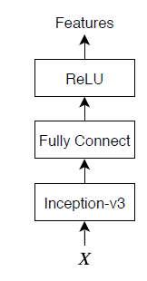
符号化器モデルは、事前学習済みの Inception-v3 モデルで、"mixed10" 層から特徴を抽出し、その後に全結合演算と ReLU 演算を行います。

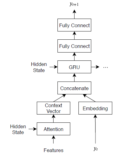
復号化器モデルは、単語埋め込み、アテンションメカニズム、ゲート付き回帰型ユニット (GRU)、および 2 つの全結合演算で構成されます。

事前学習済みのネットワークの読み込み

事前学習済みの Inception-v3 ネットワークを読み込みます。この手順には、Deep Learning Toolbox™ Model for Inception-v3 Network サポートパッケージが必要です。必要なサポートパッケージがインストールされていない場合、ダウンロード用リンクが表示されます。

net = inceptionv3;
inputSizeNet = net.Layers(1).InputSize;

特徴抽出のためにネットワークを dlnetwork オブジェクトに変換し、最後の 4 層を削除して、最後の層を "mixed10" 層にします。

lgraph = layerGraph(net);
lgraph = removeLayers(lgraph,["avg_pool" "predictions" "predictions_softmax" "ClassificationLayer_predictions"]);

ネットワークの入力層を表示します。Inception-v3 ネットワークは、最小値 0、最大値 255 の対称と再スケーリングの正規化を使用します。

lgraph.Layers(1)

ans = 
  ImageInputLayer with properties:

                      Name: 'input_1'
                 InputSize: [299 299 3]

   Hyperparameters
          DataAugmentation: 'none'
             Normalization: 'rescale-symmetric'
    NormalizationDimension: 'auto'
                       Max: 255
                       Min: 0

カスタム学習はこの正規化をサポートしません。このため、ネットワーク内の正規化を無効にして、代わりにカスタム学習ループで正規化を実行しなければなりません。最小値と最大値をそれぞれ inputMin と inputMax という名前の変数に double 型で保存し、入力層を正規化のないイメージ入力層に置き換えます。

inputMin = double(lgraph.Layers(1).Min);
inputMax = double(lgraph.Layers(1).Max);
layer = imageInputLayer(inputSizeNet,Normalization="none",Name="input");
lgraph = replaceLayer(lgraph,"input_1",layer);

ネットワークの出力サイズを決定します。関数 analyzeNetwork を使用して最後の層の活性化サイズを確認します。カスタム学習ループワークフローのネットワークを解析するには、TargetUsage オプションを "dlnetwork" に設定します。

analyzeNetwork(lgraph,TargetUsage="dlnetwork")

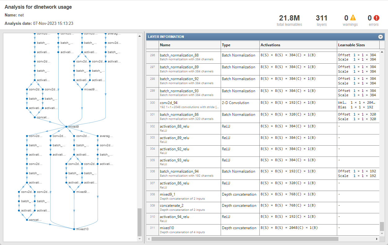
ネットワークの出力サイズを含む outputSizeNet という名前の変数を作成します。

outputSizeNet = [8 8 2048];

層グラフを dlnetwork オブジェクトに変換して出力層を表示します。出力層は Inception-v3 ネットワークの "mixed10" 層です。

net = dlnetwork(lgraph)

dlnet = 
  dlnetwork with properties:

         Layers: [311×1 nnet.cnn.layer.Layer]
    Connections: [345×2 table]
     Learnables: [376×3 table]
          State: [188×3 table]
     InputNames: {'input'}
    OutputNames: {'mixed10'}

COCO データセットのインポート

https://cocodataset.org/#download のデータセット "2014 Train images" と "2014 Train/val annotations" から、イメージと注釈をそれぞれダウンロードします。イメージと注釈を "coco" という名前のフォルダーに解凍します。COCO 2014 データセットは Coco Consortium によって収集されたものです。

関数 jsondecode を使用して、ファイル "captions_train2014.json" からキャプションを抽出します。

dataFolder = fullfile(tempdir,"coco");
filename = fullfile(dataFolder,"annotations_trainval2014","annotations","captions_train2014.json");
str = fileread(filename);
data = jsondecode(str)

data = struct with fields:
           info: [1×1 struct]
         images: [82783×1 struct]
       licenses: [8×1 struct]
    annotations: [414113×1 struct]

struct の annotations フィールドには、イメージキャプショニングに必要なデータが格納されます。

data.annotations

ans=414113×1 struct array with fields:
    image_id
    id
    caption

このデータセットにはイメージごとに複数のキャプションが格納されています。学習セットと検証セットの両方に同じイメージが出現することがないように、関数 unique を使用してデータセットにある一意のイメージを特定します。これにはデータの注釈フィールドにある image_id フィールドの ID を使用し、その後、一意のイメージの数を表示します。

numObservationsAll = numel(data.annotations)

numObservationsAll = 414113

imageIDs = [data.annotations.image_id];
imageIDsUnique = unique(imageIDs);
numUniqueImages = numel(imageIDsUnique)

numUniqueImages = 82783

各イメージに少なくとも 5 つのキャプションがあります。次のフィールドをもつ struct annotationsAll を作成します。

ImageID — イメージ ID
Filename — イメージのファイル名
Captions — 生のキャプションの string 配列
CaptionIDs — data.annotations のキャプションに対応するインデックスのベクトル

マージを容易にするために、注釈をイメージ ID で並べ替えます。

[~,idx] = sort([data.annotations.image_id]);
data.annotations = data.annotations(idx);

注釈に対してループし、必要に応じて複数の注釈をマージします。

i = 0;
j = 0;
imageIDPrev = 0;
while i < numel(data.annotations)
    i = i + 1;
    
    imageID = data.annotations(i).image_id;
    caption = string(data.annotations(i).caption);
    
    if imageID ~= imageIDPrev
        % Create new entry
        j = j + 1;
        annotationsAll(j).ImageID = imageID;
        annotationsAll(j).Filename = fullfile(dataFolder,"train2014","COCO_train2014_" + pad(string(imageID),12,"left","0") + ".jpg");
        annotationsAll(j).Captions = caption;
        annotationsAll(j).CaptionIDs = i;
    else
        % Append captions
        annotationsAll(j).Captions = [annotationsAll(j).Captions; caption];
        annotationsAll(j).CaptionIDs = [annotationsAll(j).CaptionIDs; i];
    end
    
    imageIDPrev = imageID;
end

データを学習セットと検証セットに分割します。観測値の 5% をテスト用にホールドアウトします。

cvp = cvpartition(numel(annotationsAll),HoldOut=0.05);
idxTrain = training(cvp);
idxTest = test(cvp);
annotationsTrain = annotationsAll(idxTrain);
annotationsTest = annotationsAll(idxTest);

struct には 3 つのフィールドがあります。

id — キャプションの一意の識別子
caption — イメージのキャプション。特徴ベクトルとして指定
image_id — キャプションに対応するイメージの一意の識別子

イメージと対応するキャプションを表示するには、"train2014\COCO_train2014_XXXXXXXXXXXX.jpg" というファイル名のイメージファイルを検索します。ここで、"XXXXXXXXXXXX" はゼロで左パディングして長さを 12 にしたイメージ ID に対応します。

imageID = annotationsTrain(1).ImageID;
captions = annotationsTrain(1).Captions;
filename = annotationsTrain(1).Filename;

イメージを表示するには、関数 imread と関数 imshow を使用します。

img = imread(filename);
figure
imshow(img)
title(captions)

学習用データの準備

学習用とテスト用のキャプションを準備します。学習データとテストデータ (annotationsAll) の両方を含む struct の Captions フィールドからテキストを抽出し、句読点文字を消去して、テキストを小文字に変換します。

captionsAll = cat(1,annotationsAll.Captions);
captionsAll = erasePunctuation(captionsAll);
captionsAll = lower(captionsAll);

キャプションを生成するためには、テキスト生成の開始と終了のタイミングをそれぞれ示す、特殊な開始と停止のトークンが RNN 復号化器に必要です。カスタムトークンの "<start>" と "<stop>" を、キャプションの始まりと終わりにそれぞれ追加します。

captionsAll = "<start>" + captionsAll + "<stop>";

関数 tokenizedDocument を使用してキャプションをトークン化し、CustomTokens オプションを使用して開始と停止のトークンを指定します。

documentsAll = tokenizedDocument(captionsAll,CustomTokens=["<start>" "<stop>"]);

単語と数値インデックスの間を相互にマッピングする wordEncoding オブジェクトを作成します。学習データ内で最も頻繁に観測される単語に対応する 5000 を語彙サイズに指定して、メモリ要件を減らします。バイアスを避けるには、学習セットに対応するドキュメントのみを使用します。

enc = wordEncoding(documentsAll(idxTrain),MaxNumWords=5000,Order="frequency");

キャプションに対応するイメージを含む拡張イメージデータストアを作成します。畳み込みネットワークの入力サイズに一致する出力サイズを設定します。イメージとキャプションの同期を保持するために、イメージ ID を使用してファイル名を再構成し、データストアにファイル名のテーブルを指定します。グレースケールイメージを 3 チャネルの RGB イメージに戻すために、ColorPreprocessing オプションを "gray2rgb" に設定します。

tblFilenames = table(cat(1,annotationsTrain.Filename));
augimdsTrain = augmentedImageDatastore(inputSizeNet,tblFilenames,ColorPreprocessing="gray2rgb")

augimdsTrain = 
  augmentedImageDatastore with properties:

         NumObservations: 78644
           MiniBatchSize: 1
        DataAugmentation: 'none'
      ColorPreprocessing: 'gray2rgb'
              OutputSize: [299 299]
          OutputSizeMode: 'resize'
    DispatchInBackground: 0

モデルパラメーターの初期化

モデルパラメーターを初期化します。256 の単語埋め込み次元をもつ、512 個の隠れユニットを指定します。

embeddingDimension = 256;
numHiddenUnits = 512;

符号化器モデルのパラメーターを含む struct を初期化します。

この例の最後にリストされている関数 initializeGlorot で指定される Glorot 初期化子を使用して、全結合演算の重みを初期化します。出力サイズを復号化器の埋め込み次元 (256) に一致するように、また入力サイズを事前学習済みネットワークの出力チャネル数に一致するように指定します。Inception-v3 ネットワークの 'mixed10' 層は 2048 チャネルのデータを出力します。

numFeatures = outputSizeNet(1) * outputSizeNet(2);
inputSizeEncoder = outputSizeNet(3);
parametersEncoder = struct;

% Fully connect
parametersEncoder.fc.Weights = dlarray(initializeGlorot(embeddingDimension,inputSizeEncoder));
parametersEncoder.fc.Bias = dlarray(zeros([embeddingDimension 1],"single"));

復号化器モデルのパラメーターを含む struct を初期化します。

埋め込み次元と語彙サイズに 1 を加えた数で与えられるサイズで単語埋め込みの重みを初期化します。ここで、追加のエントリはパディング値に対応します。
GRU 演算の隠れユニット数に対応するサイズで Bahdanau アテンションメカニズムのための重みとバイアスを初期化します。
GRU 演算の重みとバイアスを初期化します。
2 つの全結合演算の重みとバイアスを初期化します。

モデル復号化器パラメーターについて、個々の重みとバイアスを Glorot 初期化子とゼロでそれぞれ初期化します。

inputSizeDecoder = enc.NumWords + 1;
parametersDecoder = struct;

% Word embedding
parametersDecoder.emb.Weights = dlarray(initializeGlorot(embeddingDimension,inputSizeDecoder));

% Attention
parametersDecoder.attention.Weights1 = dlarray(initializeGlorot(numHiddenUnits,embeddingDimension));
parametersDecoder.attention.Bias1 = dlarray(zeros([numHiddenUnits 1],"single"));
parametersDecoder.attention.Weights2 = dlarray(initializeGlorot(numHiddenUnits,numHiddenUnits));
parametersDecoder.attention.Bias2 = dlarray(zeros([numHiddenUnits 1],"single"));
parametersDecoder.attention.WeightsV = dlarray(initializeGlorot(1,numHiddenUnits));
parametersDecoder.attention.BiasV = dlarray(zeros(1,1,"single"));

% GRU
parametersDecoder.gru.InputWeights = dlarray(initializeGlorot(3*numHiddenUnits,2*embeddingDimension));
parametersDecoder.gru.RecurrentWeights = dlarray(initializeGlorot(3*numHiddenUnits,numHiddenUnits));
parametersDecoder.gru.Bias = dlarray(zeros(3*numHiddenUnits,1,"single"));

% Fully connect
parametersDecoder.fc1.Weights = dlarray(initializeGlorot(numHiddenUnits,numHiddenUnits));
parametersDecoder.fc1.Bias = dlarray(zeros([numHiddenUnits 1],"single"));

% Fully connect
parametersDecoder.fc2.Weights = dlarray(initializeGlorot(enc.NumWords+1,numHiddenUnits));
parametersDecoder.fc2.Bias = dlarray(zeros([enc.NumWords+1 1],"single"));

モデルの関数の定義

この例の最後にリストされている関数 modelEncoder および modelDecoder を作成し、符号化器および復号化器モデルの出力をそれぞれ計算します。

この例の符号化器モデル関数の節にリストされている関数 modelEncoder は、事前学習済みネットワークの出力から活性化の配列 X を入力として受け取り、全結合演算と ReLU 演算に渡します。事前学習済みネットワークは自動微分のトレースをする必要がないため、符号化器モデル関数の外で特徴を抽出するほうが効率的に計算できます。

この例の復号化器モデル関数の節にリストされている関数 modelDecoder は、入力単語に対応する単一の入力タイムステップ、復号化器モデルパラメーター、符号化器からの特徴、およびネットワーク状態を入力として受け取り、次のタイムステップの予測、更新されたネットワーク状態、およびアテンションの重みを返します。

学習オプションの指定

学習用のオプションを指定します。ミニバッチサイズ 128 で 30 エポック学習させ、学習の進行状況をプロットに表示します。

miniBatchSize = 128;
numEpochs = 30;
plots = "training-progress";

GPU が利用できる場合、GPU で学習を行います。GPU を使用するには、Parallel Computing Toolbox™ とサポートされている GPU デバイスが必要です。サポートされているデバイスについては、GPU 計算の要件 (Parallel Computing Toolbox)を参照してください。

executionEnvironment = "auto";

ネットワークの学習

カスタム学習ループを使用してネットワークに学習させます。

各エポックの始めに入力データをシャッフルします。拡張イメージデータストア内のイメージとキャプションの同期を保つために、両方のデータセットにインデックス付けする、シャッフルされたインデックスの配列を作成します。

各ミニバッチで次を行います。

事前学習済みネットワークに必要なサイズにイメージを再スケーリングします。
各イメージについて、ランダムなキャプションを選択します。
キャプションを単語インデックスのシーケンスに変換します。シーケンスの右パディングに、パディングトークンのインデックスに対応するパディング値を指定します。
データを dlarray オブジェクトに変換します。イメージについて、次元ラベル "SSCB" (spatial、spatial、channel、batch) を指定します。
GPU での学習用に、データを gpuArray オブジェクトに変換します。
事前学習済みのネットワークを使用してイメージの特徴を抽出し、符号化器で必要なサイズに形状を変更します。
関数 dlfeval および modelLoss を使用してモデルの損失と勾配を評価します。
関数 adamupdate を使用して符号化器および復号化器のモデルパラメーターを更新します。
学習の進行状況をプロットに表示します。

Adam オプティマイザーのパラメーターを初期化します。

trailingAvgEncoder = [];
trailingAvgSqEncoder = [];

trailingAvgDecoder = [];
trailingAvgSqDecoder = [];

学習の進行状況プロットを初期化します。対応する反復に対する損失をプロットする、アニメーションの線を作成します。

if plots == "training-progress"
    figure
    lineLossTrain = animatedline(Color=[0.85 0.325 0.098]);
    xlabel("Iteration")
    ylabel("Loss")
    ylim([0 inf])
    grid on
end

モデルに学習させます。

iteration = 0;
numObservationsTrain = numel(annotationsTrain);
numIterationsPerEpoch = floor(numObservationsTrain / miniBatchSize);
start = tic;

% Loop over epochs.
for epoch = 1:numEpochs
    
    % Shuffle data.
    idxShuffle = randperm(numObservationsTrain);
    
    % Loop over mini-batches.
    for i = 1:numIterationsPerEpoch
        iteration = iteration + 1;
        
        % Determine mini-batch indices.
        idx = (i-1)*miniBatchSize+1:i*miniBatchSize;
        idxMiniBatch = idxShuffle(idx);
        
        % Read mini-batch of data.
        tbl = readByIndex(augimdsTrain,idxMiniBatch);
        X = cat(4,tbl.input{:});
        annotations = annotationsTrain(idxMiniBatch);
        
        % For each image, select random caption.
        idx = cellfun(@(captionIDs) randsample(captionIDs,1),{annotations.CaptionIDs});
        documents = documentsAll(idx);
        
        % Create batch of data.
        [X, T] = createBatch(X,documents,net,inputMin,inputMax,enc,executionEnvironment);
        
        % Evaluate the model loss and gradients using dlfeval and the
        % modelLoss function.
        [loss, gradientsEncoder, gradientsDecoder] = dlfeval(@modelLoss, parametersEncoder, ...
            parametersDecoder, X, T);
        
        % Update encoder using adamupdate.
        [parametersEncoder, trailingAvgEncoder, trailingAvgSqEncoder] = adamupdate(parametersEncoder, ...
            gradientsEncoder, trailingAvgEncoder, trailingAvgSqEncoder, iteration);
        
        % Update decoder using adamupdate.
        [parametersDecoder, trailingAvgDecoder, trailingAvgSqDecoder] = adamupdate(parametersDecoder, ...
            gradientsDecoder, trailingAvgDecoder, trailingAvgSqDecoder, iteration);
        
        % Display the training progress.
        if plots == "training-progress"
            D = duration(0,0,toc(start),Format="hh:mm:ss");
            addpoints(lineLossTrain,iteration,double(loss))
            title("Epoch: " + epoch + ", Elapsed: " + string(D))
            
            drawnow
        end
    end
end

新しいキャプションの予測

キャプション生成のプロセスは、学習のためのプロセスと異なります。学習中には、復号化器は、各タイムステップで前のタイムステップにおける真の値を入力として使用します。これは "教師強制" と呼ばれます。新しいデータの予測を行うとき、復号化器は真の値の代わりに前の予測値を使用します。

シーケンスの各ステップで最も有力な単語を予測することが、準最適の結果につながる可能性があります。たとえば、復号化器に象のイメージが与えられて、キャプションの最初の単語が "a" と予測された場合、英語のテキストに "a elephant" というフレーズが出現する可能性は極端に低いため、次の単語として "elephant" が予測される可能性は大幅に低くなります。

この問題に対処するために、ビームサーチアルゴリズムを使用できます。シーケンスの各ステップで最も有力な予測を選ぶのではなく、上位 k 個の予測 (ビームインデックス) を選び、後続の各ステップで全体のスコアに従って、これまでの上位 k 個の予測シーケンスを保持します。

新しいイメージのキャプションを生成するには、イメージの特徴を抽出し、符号化器に入力した後で、この例のビームサーチ関数の節にリストされている関数 beamSearch を使用します。

img = imread("laika_sitting.jpg");
X = extractImageFeatures(net,img,inputMin,inputMax,executionEnvironment);

beamIndex = 3;
maxNumWords = 20;
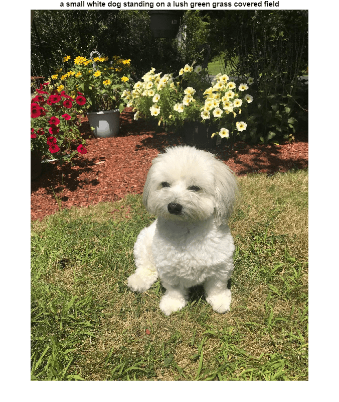
[words,attentionScores] = beamSearch(X,beamIndex,parametersEncoder,parametersDecoder,enc,maxNumWords);
caption = join(words)

caption = 
"a dog is standing on a tile floor"

イメージをキャプションと共に表示します。

figure
imshow(img)
title(caption)

データセットのキャプションの予測

イメージコレクションのキャプションを予測するために、データストア内のデータのミニバッチをループ処理し、関数 extractImageFeatures を使用してイメージから特徴を抽出します。次に、ミニバッチのイメージをループ処理し、関数 beamSearch を使用してキャプションを生成します。

拡張イメージデータストアを作成して、畳み込みネットワークの入力サイズに一致するように出力サイズを設定します。グレースケールイメージを 3 チャネルの RGB イメージとして出力するために、ColorPreprocessing オプションを "gray2rgb" に設定します。

tblFilenamesTest = table(cat(1,annotationsTest.Filename));
augimdsTest = augmentedImageDatastore(inputSizeNet,tblFilenamesTest,ColorPreprocessing="gray2rgb")

augimdsTest = 
  augmentedImageDatastore with properties:

         NumObservations: 4139
           MiniBatchSize: 1
        DataAugmentation: 'none'
      ColorPreprocessing: 'gray2rgb'
              OutputSize: [299 299]
          OutputSizeMode: 'resize'
    DispatchInBackground: 0

テストデータのキャプションを生成します。大きなデータセットでのキャプションの予測には時間がかかる場合があります。Parallel Computing Toolbox™ がある場合、キャプションを parfor ループの中で生成することによって、並列で予測を行えます。Parallel Computing Toolbox がない場合は、parfor ループは逐次実行されます。

beamIndex = 2;
maxNumWords = 20;

numObservationsTest = numel(annotationsTest);
numIterationsTest = ceil(numObservationsTest/miniBatchSize);

captionsTestPred = strings(1,numObservationsTest);
documentsTestPred = tokenizedDocument(strings(1,numObservationsTest));

for i = 1:numIterationsTest
    % Mini-batch indices.
    idxStart = (i-1)*miniBatchSize+1;
    idxEnd = min(i*miniBatchSize,numObservationsTest);
    idx = idxStart:idxEnd;
    
    sz = numel(idx);
    
    % Read images.
    tbl = readByIndex(augimdsTest,idx);
    
    % Extract image features.
    X = cat(4,tbl.input{:});
    X = extractImageFeatures(net,X,inputMin,inputMax,executionEnvironment);
    
    % Generate captions.
    captionsPredMiniBatch = strings(1,sz);
    documentsPredMiniBatch = tokenizedDocument(strings(1,sz));
    
    parfor j = 1:sz
        words = beamSearch(X(:,:,j),beamIndex,parametersEncoder,parametersDecoder,enc,maxNumWords);
        captionsPredMiniBatch(j) = join(words);
        documentsPredMiniBatch(j) = tokenizedDocument(words,TokenizeMethod="none");
    end
    
    captionsTestPred(idx) = captionsPredMiniBatch;
    documentsTestPred(idx) = documentsPredMiniBatch;
end

Analyzing and transferring files to the workers ...done.

テストイメージを、対応するキャプションと合わせて表示するには、関数 imshow を使用してタイトルを予測されたキャプションに設定します。

idx = 1;
tbl = readByIndex(augimdsTest,idx);
img = tbl.input{1};
figure
imshow(img)
title(captionsTestPred(idx))

モデルの精度の評価

BLEU スコアを使用してキャプションの精度を評価するには、関数 bleuEvaluationScore を用いて各キャプション (候補) をその対応するテストセット内のキャプション (参照) と比べて BLEU スコアを計算します。関数 bleuEvaluationScore を使用すると、単一の候補ドキュメントを複数の参照ドキュメントと比較できます。

関数 bleuEvaluationScore は、既定では長さが 1 から 4 の n-gram を使用して類似度のスコアを計算します。キャプションは短いため、この動作ではほとんどのスコアがゼロに近くなり、情報価値のない結果につながります。NgramWeights オプションを重みの等しい 2 要素ベクトルに設定することで、n-gram の長さを 1 から 2 に設定します。

ngramWeights = [0.5 0.5];

for i = 1:numObservationsTest
    annotation = annotationsTest(i);
    
    captionIDs = annotation.CaptionIDs;
    candidate = documentsTestPred(i);
    references = documentsAll(captionIDs);
    
    score = bleuEvaluationScore(candidate,references,NgramWeights=ngramWeights);
    
    scores(i) = score;
end

平均の BLEU スコアを表示します。

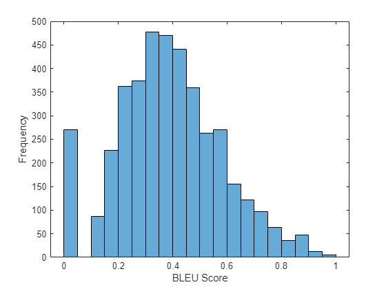
scoreMean = mean(scores)

scoreMean = 0.4224

ヒストグラムでスコアを可視化します。

figure
histogram(scores)
xlabel("BLEU Score")
ylabel("Frequency")

アテンション関数

関数 attention は、Bahdanau アテンションを使用してコンテキストベクトルとアテンションの重みを計算します。

function [contextVector, attentionWeights] = attention(hidden,features,weights1, ...
    bias1,weights2,bias2,weightsV,biasV)

% Model dimensions.
[embeddingDimension,numFeatures,miniBatchSize] = size(features);
numHiddenUnits = size(weights1,1);

% Fully connect.
Y1 = reshape(features,embeddingDimension, numFeatures*miniBatchSize);
Y1 = fullyconnect(Y1,weights1,bias1,DataFormat="CB");
Y1 = reshape(Y1,numHiddenUnits,numFeatures,miniBatchSize);

% Fully connect.
Y2 = fullyconnect(hidden,weights2,bias2,DataFormat="CB");
Y2 = reshape(Y2,numHiddenUnits,1,miniBatchSize);

% Addition, tanh.
scores = tanh(Y1 + Y2);
scores = reshape(scores, numHiddenUnits, numFeatures*miniBatchSize);

% Fully connect, softmax.
attentionWeights = fullyconnect(scores,weightsV,biasV,DataFormat="CB");
attentionWeights = reshape(attentionWeights,1,numFeatures,miniBatchSize);
attentionWeights = softmax(attentionWeights,DataFormat="SCB");

% Context.
contextVector = attentionWeights .* features;
contextVector = squeeze(sum(contextVector,2));

end

埋め込み関数

関数 embedding は、インデックスの配列を、埋め込みベクトルのシーケンスにマッピングします。

function Z = embedding(X, weights)

% Reshape inputs into a vector
[N, T] = size(X, 1:2);
X = reshape(X, N*T, 1);

% Index into embedding matrix
Z = weights(:, X);

% Reshape outputs by separating out batch and sequence dimensions
Z = reshape(Z, [], N, T);

end

特徴抽出関数

関数 extractImageFeatures は、学習済みの dlnetwork オブジェクト、入力イメージ、イメージ再スケーリングの統計、および実行環境を入力として受け取り、事前学習済みのネットワークから抽出した特徴を含む dlarray を返します。

function X = extractImageFeatures(net,X,inputMin,inputMax,executionEnvironment)

% Resize and rescale.
inputSize = net.Layers(1).InputSize(1:2);
X = imresize(X,inputSize);
X = rescale(X,-1,1,InputMin=inputMin,InputMax=inputMax);

% Convert to dlarray.
X = dlarray(X,"SSCB");

% Convert to gpuArray.
if (executionEnvironment == "auto" && canUseGPU) || executionEnvironment == "gpu"
    X = gpuArray(X);
end

% Extract features and reshape.
X = predict(net,X);
sz = size(X);
numFeatures = sz(1) * sz(2);
inputSizeEncoder = sz(3);
miniBatchSize = sz(4);
X = reshape(X,[numFeatures inputSizeEncoder miniBatchSize]);

end

バッチ作成関数

関数 createBatch は、データのミニバッチ、トークン化されたキャプション、事前学習済みのネットワーク、イメージ再スケーリングの統計、単語符号化、および実行環境を入力として受け取り、学習用に抽出されたイメージの特徴とキャプションに対応するデータのミニバッチを返します。

function [X, T] = createBatch(X,documents,net,inputMin,inputMax,enc,executionEnvironment)

X = extractImageFeatures(net,X,inputMin,inputMax,executionEnvironment);

% Convert documents to sequences of word indices.
T = doc2sequence(enc,documents,PaddingDirection="right",PaddingValue=enc.NumWords+1);
T = cat(1,T{:});

% Convert mini-batch of data to dlarray.
T = dlarray(T);

% If training on a GPU, then convert data to gpuArray.
if (executionEnvironment == "auto" && canUseGPU) || executionEnvironment == "gpu"
    T = gpuArray(T);
end

end

符号化器モデル関数

関数 modelEncoder は、活性化の配列 X を入力として受け取り、全結合演算と ReLU 演算に渡します。全結合演算は、チャネル次元だけに対して操作を行います。チャネル次元にのみ全結合演算を適用するには、他のチャネルを単一の次元にフラット化し、関数 fullyconnect の DataFormat オプションを用いてこの次元をバッチ次元として指定します。

function Y = modelEncoder(X,parametersEncoder)

[numFeatures,inputSizeEncoder,miniBatchSize] = size(X);

% Fully connect
weights = parametersEncoder.fc.Weights;
bias = parametersEncoder.fc.Bias;
embeddingDimension = size(weights,1);

X = permute(X,[2 1 3]);
X = reshape(X,inputSizeEncoder,numFeatures*miniBatchSize);
Y = fullyconnect(X,weights,bias,DataFormat="CB");
Y = reshape(Y,embeddingDimension,numFeatures,miniBatchSize);

% ReLU
Y = relu(Y);

end

復号化器モデル関数

関数 modelDecoder は、単一タイムステップ X、復号化器モデルパラメーター、符号化器からの特徴、およびネットワーク状態を入力として受け取り、次のタイムステップ用の予測、更新されたネットワーク状態、およびアテンションの重みを返します。

function [Y,state,attentionWeights] = modelDecoder(X,parametersDecoder,features,state)

hiddenState = state.gru.HiddenState;

% Attention
weights1 = parametersDecoder.attention.Weights1;
bias1 = parametersDecoder.attention.Bias1;
weights2 = parametersDecoder.attention.Weights2;
bias2 = parametersDecoder.attention.Bias2;
weightsV = parametersDecoder.attention.WeightsV;
biasV = parametersDecoder.attention.BiasV;
[contextVector, attentionWeights] = attention(hiddenState,features,weights1,bias1,weights2,bias2,weightsV,biasV);

% Embedding
weights = parametersDecoder.emb.Weights;
X = embedding(X,weights);

% Concatenate
Y = cat(1,contextVector,X);

% GRU
inputWeights = parametersDecoder.gru.InputWeights;
recurrentWeights = parametersDecoder.gru.RecurrentWeights;
bias = parametersDecoder.gru.Bias;
[Y, hiddenState] = gru(Y, hiddenState, inputWeights, recurrentWeights, bias, DataFormat="CBT");

% Update state
state.gru.HiddenState = hiddenState;

% Fully connect
weights = parametersDecoder.fc1.Weights;
bias = parametersDecoder.fc1.Bias;
Y = fullyconnect(Y,weights,bias,DataFormat="CB");

% Fully connect
weights = parametersDecoder.fc2.Weights;
bias = parametersDecoder.fc2.Bias;
Y = fullyconnect(Y,weights,bias,DataFormat="CB");

end

モデルの損失

関数 modelLoss は、符号化器と復号化器のパラメーター、符号化器の特徴 X、およびターゲットのキャプション T を入力として受け取り、損失、その損失についての符号化器と復号化器のパラメーターの勾配、および予測を返します。

function [loss,gradientsEncoder,gradientsDecoder,YPred] = ...
    modelLoss(parametersEncoder,parametersDecoder,X,T)

miniBatchSize = size(X,3);
sequenceLength = size(T,2) - 1;
vocabSize = size(parametersDecoder.emb.Weights,2);

% Model encoder
features = modelEncoder(X,parametersEncoder);

% Initialize state
numHiddenUnits = size(parametersDecoder.attention.Weights1,1);
state = struct;
state.gru.HiddenState = dlarray(zeros([numHiddenUnits miniBatchSize],"single"));

YPred = dlarray(zeros([vocabSize miniBatchSize sequenceLength],"like",X));
loss = dlarray(single(0));

padToken = vocabSize;

for t = 1:sequenceLength
    decoderInput = T(:,t);
    
    YReal = T(:,t+1);
    
    [YPred(:,:,t),state] = modelDecoder(decoderInput,parametersDecoder,features,state);
    
    mask = YReal ~= padToken;
    
    loss = loss + sparseCrossEntropyAndSoftmax(YPred(:,:,t),YReal,mask);
end

% Calculate gradients
[gradientsEncoder,gradientsDecoder] = dlgradient(loss, parametersEncoder,parametersDecoder);

end

スパースな交差エントロピーおよびソフトマックス損失関数

関数 sparseCrossEntropyAndSoftmax は、予測 Y、対応するターゲット T、およびシーケンスパディングマスクを入力として受け取り、関数 softmax を適用して交差エントロピー損失を返します。

function loss = sparseCrossEntropyAndSoftmax(Y, T, mask)

miniBatchSize = size(Y, 2);

% Softmax.
Y = softmax(Y,DataFormat="CB");

% Find rows corresponding to the target words.
idx = sub2ind(size(Y), T', 1:miniBatchSize);
Y = Y(idx);

% Bound away from zero.
Y = max(Y, single(1e-8));

% Masked loss.
loss = log(Y) .* mask';
loss = -sum(loss,"all") ./ miniBatchSize;

end

ビームサーチ関数

関数 beamSearch は、イメージの特徴 X、ビームインデックス、符号化器ネットワークおよび復号化器ネットワークのパラメーター、単語符号化、および最大シーケンス長を入力として受け取り、ビームサーチアルゴリズムを使用してイメージのキャプション用の単語を返します。

function [words,attentionScores] = beamSearch(X,beamIndex,parametersEncoder,parametersDecoder, ...
    enc,maxNumWords)

% Model dimensions
numFeatures = size(X,1);
numHiddenUnits = size(parametersDecoder.attention.Weights1,1);

% Extract features
features = modelEncoder(X,parametersEncoder);

% Initialize state
state = struct;
state.gru.HiddenState = dlarray(zeros([numHiddenUnits 1],"like",X));

% Initialize candidates
candidates = struct;
candidates.State = state;
candidates.Words = "<start>";
candidates.Score = 0;
candidates.AttentionScores = dlarray(zeros([numFeatures maxNumWords],"like",X));
candidates.StopFlag = false;

t = 0;

% Loop over words
while t < maxNumWords
    t = t + 1;
    
    candidatesNew = [];
    
    % Loop over candidates
    for i = 1:numel(candidates)
        
        % Stop generating when stop token is predicted
        if candidates(i).StopFlag
            continue
        end
        
        % Candidate details
        state = candidates(i).State;
        words = candidates(i).Words;
        score = candidates(i).Score;
        attentionScores = candidates(i).AttentionScores;
        
        % Predict next token
        decoderInput = word2ind(enc,words(end));
        [YPred,state,attentionScores(:,t)] = modelDecoder(decoderInput,parametersDecoder,features,state);
        
        YPred = softmax(YPred,DataFormat="CB");
        [scoresTop,idxTop] = maxk(extractdata(YPred),beamIndex);
        idxTop = gather(idxTop);
        
        % Loop over top predictions
        for j = 1:beamIndex
            candidate = struct;
            
            candidateWord = ind2word(enc,idxTop(j));
            candidateScore = scoresTop(j);
            
            if candidateWord == "<stop>"
                candidate.StopFlag = true;
                attentionScores(:,t+1:end) = [];
            else
                candidate.StopFlag = false;
            end
            
            candidate.State = state;
            candidate.Words = [words candidateWord];
            candidate.Score = score + log(candidateScore);
            candidate.AttentionScores = attentionScores;
            
            candidatesNew = [candidatesNew candidate];
        end
    end
    
    % Get top candidates
    [~,idx] = maxk([candidatesNew.Score],beamIndex);
    candidates = candidatesNew(idx);
    
    % Stop predicting when all candidates have stop token
    if all([candidates.StopFlag])
        break
    end
end

% Get top candidate
words = candidates(1).Words(2:end-1);
attentionScores = candidates(1).AttentionScores;

end

Glorot 重み初期化関数

関数 initializeGlorot は、Glorot の初期化に従って、重みの配列を生成します。

function weights = initializeGlorot(numOut, numIn)

varWeights = sqrt( 6 / (numIn + numOut) );
weights = varWeights * (2 * rand([numOut, numIn], "single") - 1);

end

参考

アテンションを使用したイメージ キャプションの生成