lqr

Linear-Quadratic Regulator (LQR) design

Syntax

[K,S,P] = lqr(sys,Q,R,N)

[K,S,P] = lqr(A,B,Q,R,N)

Description

[K,S,P] = lqr(sys,Q,R,N) calculates the optimal gain matrix K, the solution S of the associated algebraic Riccati equation, and the closed-loop poles P for the continuous-time or discrete-time state-space model sys. Q and R are the weight matrices for states and inputs, respectively. The cross term matrix N is set to zero when omitted.

[K,S,P] = lqr(A,B,Q,R,N) calculates the optimal gain matrix K, the solution S of the associated algebraic Riccati equation and the closed-loop poles P using the continuous-time state-space matrices A and B. This syntax is only valid for continuous-time models. For discrete-time models, use dlqr.

Examples

LQR Control for Inverted Pendulum Model

pendulumModelCart.mat contains the state-space model of an inverted pendulum on a cart where the outputs are the cart displacement x and the pendulum angle $\theta$. The control input u is the horizontal force on the cart.

$$\begin{array}{l}\left[\begin{array}{c}\underset{}{\overset{\dot{}}{x}}\\ \underset{}{\overset{¨}{x}}\\ \underset{}{\overset{\dot{}}{\theta }}\\ \underset{}{\overset{¨}{\theta }}\end{array}\right]=\left[\begin{array}{cccc}0& 1& 0& 0\\ 0& -0.1& 3& 0\\ 0& 0& 0& 1\\ 0& -0.5& 30& 0\end{array}\right]\left[\begin{array}{c}x\\ \underset{}{\overset{\dot{}}{x}}\\ \theta \\ \underset{}{\overset{\dot{}}{\theta }}\end{array}\right]+\left[\begin{array}{c}0\\ 2\\ 0\\ 5\end{array}\right]u\\ y=\left[\begin{array}{cccc}1& 0& 0& 0\\ 0& 0& 1& 0\end{array}\right]\left[\begin{array}{c}x\\ \underset{}{\overset{\dot{}}{x}}\\ \theta \\ \underset{}{\overset{\dot{}}{\theta }}\end{array}\right]+\left[\begin{array}{c}0\\ 0\end{array}\right]u\end{array}$$

First, load the state-space model sys to the workspace.

load('pendulumCartModel.mat','sys')

Since the outputs are x and $\theta$, and there is only one input, use Bryson's rule to determine Q and R.

Q = [1,0,0,0;...
    0,0,0,0;...
    0,0,1,0;...
    0,0,0,0];
R = 1;

Find the gain matrix K using lqr. Since N is not specified, lqr sets N to 0.

[K,S,P] = lqr(sys,Q,R)

K = 1×4

   -1.0000   -1.7559   16.9145    3.2274

S = 4×4

    1.5346    1.2127   -3.2274   -0.6851
    1.2127    1.5321   -4.5626   -0.9640
   -3.2274   -4.5626   26.5487    5.2079
   -0.6851   -0.9640    5.2079    1.0311

P = 4×1 complex

  -0.8684 + 0.8523i
  -0.8684 - 0.8523i
  -5.4941 + 0.4564i
  -5.4941 - 0.4564i

Although Bryson's rule usually provides satisfactory results, it is often just the starting point of a trial-and-error iterative design procedure to tune your closed-loop system response based on the design requirements.

LQR Control Using State-Space Matrices

aircraftPitchModel.mat contains the state-space matrices of an aircraft where the input is the elevator deflection angle $\delta$ and the output is the aircraft pitch angle $\theta$.

$$\begin{array}{l}\left[\begin{array}{c}\underset{}{\overset{\dot{}}{\alpha }}\\ \underset{}{\overset{\dot{}}{q}}\\ \underset{}{\overset{\dot{}}{\theta }}\end{array}\right]=\left[\begin{array}{ccc}-0.313& 56.7& 0\\ -0.0139& -0.426& 0\\ 0& 56.7& 0\end{array}\right]\left[\begin{array}{c}\alpha \\ q\\ \theta \end{array}\right]+\left[\begin{array}{c}0.232\\ 0.0203\\ 0\end{array}\right]\left[\delta \right]\\ y=\left[\begin{array}{ccc}0& 0& 1\end{array}\right]\left[\begin{array}{c}\alpha \\ q\\ \theta \end{array}\right]+\left[0\right]\left[\delta \right]\end{array}$$

For a step reference of 0.2 radians, consider the following design criteria:

• Rise time less than 2 seconds

• Settling time less than 10 seconds

• Steady-state error less than 2%

Load the model data to the workspace.

load('aircraftPitchModel.mat')

Define the state-cost weighted matrix Q and the control weighted matrix R. Generally, you can use Bryson's Rule to define your initial weighted matrices Q and R. For this example, consider the output vector C along with a scaling factor of 2 for matrix Q and choose R as 1. R is a scalar since the system has only one input.

R = 1

R = 1

Q1 = 2*C'*C

Q1 = 3×3

     0     0     0
     0     0     0
     0     0     2

Compute the gain matrix using lqr.

[K1,S1,P1] = lqr(A,B,Q1,R);

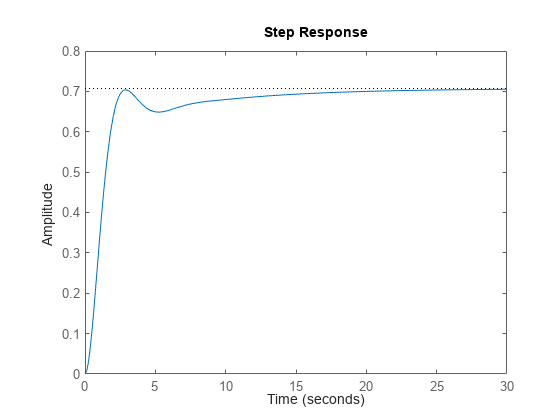
Check the closed-loop step response with the generated gain matrix K1.

sys1 = ss(A-B*K1,B,C,D);
step(sys1)

Since this response does not meet the design goals, increase the scaling factor to 25, compute the gain matrix K2, and check the closed-loop step response for gain matrix K2.

Q2 = 25*C'*C

Q2 = 3×3

     0     0     0
     0     0     0
     0     0    25

[K2,S2,P2] = lqr(A,B,Q2,R);
sys2 = ss(A-B*K2,B,C,D);
step(sys2)

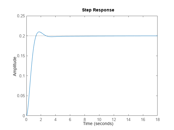
In the closed-loop step response plot, the rise time, settling time, and steady-state error meet the design goals.

Input Arguments

sys — Dynamic system model

ss model object

Dynamic system model, specified as an ss model object.

A — State matrix

n-by-n matrix

State matrix, specified as an n-by-n matrix, where n is the number of states.

B — Input-to-state matrix

n-by-m matrix

Input-to-state matrix, specified as an n-by-m input-to-state matrix, where m is the number of inputs.

Q — State-cost weighted matrix

matrix

State-cost weighted matrix, specified as an n-by-n matrix, where n is the number of states. You can use Bryson's rule to set the initial values of Q given by:

$$\begin{array}{l}{Q}_{i,i}=\frac{1}{\text{maximum acceptable value of }{\left(erro{r}_{states}\right)}^2},\text{ i}\in \left\{1,2,\mathrm{...},n\right\}\\ Q=\left[\begin{array}{cccc}{Q}_{1,1}& 0& \cdots & 0\\ 0& Q_{2,2}& \cdots & 0\\ 0& 0& \ddots & ⋮\\ 0& 0& \cdots & Q_{n,n}\end{array}\right]\end{array}$$

Here, n is the number of states.

R — Input-cost weighted matrix

scalar | matrix

Input-cost weighted matrix, specified as a scalar or a matrix of the same size as D'D. Here, D is the feed-through state-space matrix. You can use Bryson's rule to set the initial values of R given by:

$$\begin{array}{l}{R}_{j,j}=\frac{1}{\text{maximum acceptable value of }{\left(erro{r}_{inputs}\right)}^2},\text{ j}\in \left\{1,2,\mathrm{...},m\right\}\\ R=\left[\begin{array}{cccc}{R}_{1,1}& 0& \cdots & 0\\ 0& R_{2,2}& \cdots & 0\\ 0& 0& \ddots & ⋮\\ 0& 0& \cdots & R_{m,m}\end{array}\right]\end{array}$$

Here, m is the number of inputs.

N — Optional cross term matrix

0 (default) | matrix

Optional cross term matrix, specified as a matrix. If N is not specified, then lqr sets N to 0 by default.

Output Arguments

K — Optimal gain

row vector

Optimal gain of the closed-loop system, returned as a row vector of size n, where n is the number of states.

S — Solution of the associated algebraic Riccati equation

matrix

Solution of the associated algebraic Riccati equation, returned as an n-by-n matrix, where n is the number of states. In other words, S is the same dimension as state-space matrix A. For more information, see icare and idare.

P — Poles of the closed-loop system

column vector

Poles of the closed-loop system, returned as a column vector of size n, where n is the number of states.

Limitations

The input data must satisfy the following conditions:

• The pair (A,B) must be stabilizable.

• R must be positive definite.

• $$\left[\begin{array}{cc}Q& N\\ N^T& R\end{array}\right]$$ must be positive semidefinite (equivalently, $$Q-N{R}^{-1}{N}^T\ge 0$$).

• $$(Q-N{R}^{-1}{N}^T,A-B{R}^{-1}{N}^T)$$ must have no unobservable mode on the imaginary axis (or unit circle in discrete time).

Tips

• lqr supports descriptor models with nonsingular E. The output S of lqr is the solution of the algebraic Riccati equation for the equivalent explicit state-space model:

  $$\frac{dx}{dt}=E^{-1}Ax+E^{-1}Bu$$

Algorithms

For continuous-time systems, lqr computes the state-feedback control $$u=-Kx$$ that minimizes the quadratic cost function

$$J(u)={\displaystyle {\int }_0^{\infty }(x^{T}Qx+u^{T}Ru+2x^{T}Nu)dt}$$

subject to the system dynamics $$\dot{x}=Ax+Bu$$.

In addition to the state-feedback gain K, lqr returns the solution S of the associated algebraic Riccati equation

$$A^{T}S+SA-(SB+N)R^{-1}(B^{T}S+N^T)+Q=0$$

and the closed-loop poles $$P=eig\left(A-BK\right)$$. The gain matrix K is derived from S using

$$K=R^{-1}(B^{T}S+N^T).$$

For discrete-time systems, lqr computes the state-feedback control $$u_n=-K{x}_n$$ that minimizes

$$J={\displaystyle \sum _{n=0}^{\infty }\{x^{T}Qx+u^{T}Ru+2x^{T}Nu\}}$$

subject to the system dynamics $$x_{n+1}=A{x}_n+B{u}_n$$.

In all cases, when you omit the cross term matrix N, lqr sets N to 0.

Version History

Introduced before R2006a