scatterhist
周辺ヒストグラムをもつ散布図
説明
例
標本データを読み込みます。データ行列の最初の列からデータ ベクトル x を作成します。これには、アヤメの花のがく片の長さの測定値が含まれます。データ行列の 2 番目の列からデータ ベクトル y を作成します。これには、アヤメの花のがく片の幅を測定した値が含まれます。
load fisheriris
x = meas(:,1);
y = meas(:,2);
散布図と 2 つの周辺ヒストグラムを作成して、がく片の長さとがく片の幅間の関係を可視化します。
scatterhist(x,y)

ヒストグラムのビンに関するデータ ヒントを表示します。ヒストグラム内のビンにカーソルを移動すると、データ ヒントが表示されます。
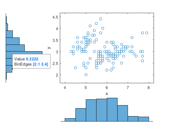
データ ヒントには、選択したビンの確率密度関数推定と、ビンのエッジの下限値および上限値が表示されます。
標本データを読み込みます。データ行列の最初の列からデータ ベクトル x を作成します。これには、3 種のアヤメの花のがく片の長さの測定値が含まれます。データ行列の 2 番目の列からデータ ベクトル y を作成します。これには、アヤメの花のがく片の幅を測定した値が含まれます。
load fisheriris.mat;
x = meas(:,1);
y = meas(:,2);
散布図と 6 つのカーネル密度プロットを作成して、がく片の長さとがく片の幅間の関係を種類別にグループ化して、可視化します。
scatterhist(x,y,'Group',species,'Kernel','on')
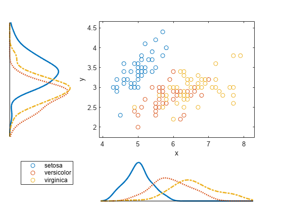
プロットには、がく片の長さとがく片の幅の関係が、花の種類に応じて異なることが示されています。
標本データを読み込みます。データ行列の最初の列からデータ ベクトル x を作成します。これには、異なる 3 種のアヤメの花のがく片の長さの測定値が含まれます。データ行列の 2 番目の列からデータ ベクトル y を作成します。これには、アヤメの花のがく片の幅を測定した値が含まれます。
load fisheriris.mat;
x = meas(:,1);
y = meas(:,2);
散布図と 6 つのカーネル密度プロットを作成して、3 種のアヤメの花で測定されたがく片の長さとがく片の幅の関係を種類別にグループ化して、可視化します。プロットの外観をカスタマイズします。
scatterhist(x,y,'Group',species,'Kernel','on','Location','SouthEast',...
    'Direction','out','Color','kbr','LineStyle',{'-','-.',':'},...
    'LineWidth',[2,2,2],'Marker','+od','MarkerSize',[4,5,6]);

標本データを読み込みます。データ行列の最初の列からデータ ベクトル x を作成します。これには、3 種のアヤメの花のがく片の長さの測定値が含まれます。データ行列の 2 番目の列からデータ ベクトル y を作成します。これには、アヤメの花のがく片の幅を測定した値が含まれます。
load fisheriris.mat;
x = meas(:,1);
y = meas(:,2);
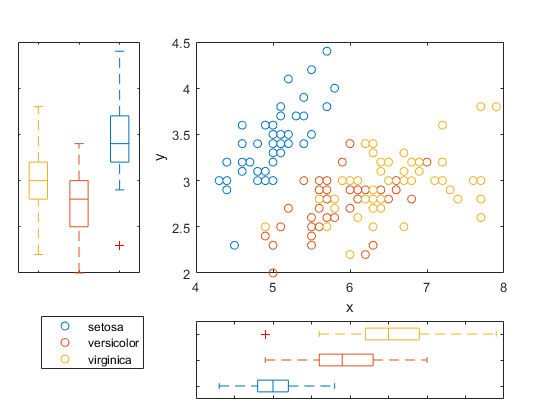
軸のハンドルを使用して、周辺ヒストグラムを箱ひげ図に置き換えます。
h = scatterhist(x,y,'Group',species);
hold on;
clr = get(h(1),'colororder');
boxplot(h(2),x,species,'orientation','horizontal',...
     'label',{'','',''},'color',clr);
boxplot(h(3),y,species,'orientation','horizontal',...
     'label', {'','',''},'color',clr);
set(h(2:3),'XTickLabel','');
view(h(3),[270,90]);  % Rotate the Y plot
axis(h(1),'auto');  % Sync axes
hold off;
標本データを読み込みます。データ行列の最初の列からデータ ベクトル x を作成します。これには、アヤメの花のがく片の長さの測定値が含まれます。データ行列の 2 番目の列からデータ ベクトル y を作成します。これには、アヤメの花のがく片の幅を測定した値が含まれます。
load fisheriris
x = meas(:,1);
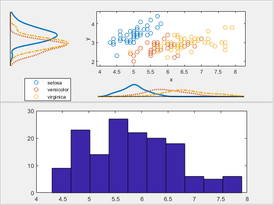
y = meas(:,2);新しく作成した図を 2 つに分割するために、2 つの uipanel オブジェクトを定義します。図の上半分では、scatterhist を使用して、標本データをプロットします。種類ごとにグループ化された周辺カーネル密度プロット図の下半分は、x に含まれるがく片の長さの測定のヒストグラムをプロットします。
figure
hp1 = uipanel('position',[0 .5 1 .5]);
hp2 = uipanel('position',[0 0 1 .5]);
scatterhist(x,y,'Group',species,'Kernel','on','Parent',hp1);
axes('Parent',hp2);
hist(x);
入力引数
名前と値の引数
出力引数
代替機能
または、関数 scatterhistogram を使用して ScatterHistogramChart オブジェクトを作成できます。
移動、ズームおよびデータ ヒントの使用により、オブジェクト内のデータを対話的に調べます。関数
scatterhistと異なり、scatterhistogramは現在の散布図の範囲内にあるデータに基づいて周辺ヒストグラムを更新します。散布ヒストグラム チャートの外観と動作を制御するには、ScatterHistogramChart のプロパティ を変更します。