KINOVA Gen3 マニピュレーターを使用した衝突のない軌跡の計画と実行

この例では、非線形モデルの予測制御を使用して、エンドエフェクタの初期姿勢から目的の姿勢まで衝突のない閉ループのロボット軌跡を計画する方法を説明します。結果の軌跡は、ジョイント空間運動モデルと計算トルク制御を使用して実行されます。障害物は静的または動的にすることができ、プリミティブ (球、円柱、ボックス) またはカスタム メッシュのいずれかとして設定できます。

ロボットの記述と姿勢

KINOVA Gen3 剛体ツリー (RBT) モデルを読み込みます。

robot = loadrobot('kinovaGen3', 'DataFormat', 'column');

ジョイントの数を取得します。

numJoints = numel(homeConfiguration(robot));

エンドエフェクタの属するロボット座標系を指定します。

endEffector = "EndEffector_Link"; 

エンドエフェクタの初期姿勢と目的の姿勢を指定します。逆運動学を使用して、指定した目的の姿勢について初期のロボット コンフィギュレーションを求めます。

% Initial end-effector pose
taskInit = trvec2tform([[0.4 0 0.2]])*axang2tform([0 1 0 pi]);

% Compute current robot joint configuration using inverse kinematics
ik = inverseKinematics('RigidBodyTree', robot);
ik.SolverParameters.AllowRandomRestart = false;
weights = [1 1 1 1 1 1];
currentRobotJConfig = ik(endEffector, taskInit, weights, robot.homeConfiguration);

% The IK solver respects joint limits, but for those joints with infinite
% range, they must be wrapped to a finite range on the interval [-pi, pi].
% Since the other joints are already bounded within this range, it is
% sufficient to simply call wrapToPi on the entire robot configuration
% rather than only on the joints with infinite range.
currentRobotJConfig = wrapToPi(currentRobotJConfig);

% Final (desired) end-effector pose
taskFinal = trvec2tform([0.35 0.55 0.35])*axang2tform([0 1 0 pi]);  
anglesFinal = rotm2eul(taskFinal(1:3,1:3),'XYZ');
poseFinal = [taskFinal(1:3,4);anglesFinal']; % 6x1 vector for final pose: [x, y, z, phi, theta, psi]

衝突メッシュと障害物

制御中に衝突をチェックして避けるには、衝突 world を一連の衝突オブジェクトとして設定しなければなりません。この例では、回避する障害物としてcollisionSphereオブジェクトを使用します。動く障害物ではなく静的な障害物を使用して計画するには、次の論理式を変更します。

isMovingObst = true;

障害物のサイズと位置は、次の補助関数で初期化されます。静的な障害物をさらに追加するには、配列 world に衝突オブジェクトを追加します。

helperCreateObstaclesKINOVA;

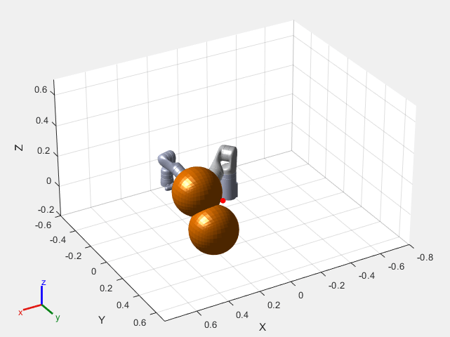
初期コンフィギュレーションでのロボットを可視化します。環境内に障害物も表示されます。

x0 = [currentRobotJConfig', zeros(1,numJoints)];
helperInitialVisualizerKINOVA;

障害物からの安全距離を指定します。この値は非線形 MPC コントローラーの不等式制約関数で使用されます。

safetyDistance = 0.01; 

非線形モデル予測コントローラーの設計

nlmpc (Model Predictive Control Toolbox)コントローラー オブジェクトを作成する次の補助ファイルを使用して、非線形モデル予測コントローラーを設計できます。ファイルを表示するには、edit helperDesignNLMPCobjKINOVA と入力します。

helperDesignNLMPCobjKINOVA;

コントローラーは次の解析に基づいて設計されます。最適化ソルバーの最大反復数は 5 に設定されます。ジョイントの位置および速度 (状態) の下限と上限、および加速度 (制御入力) は明示的に設定されます。

• ロボットのジョイント モデルは double の積分器によって記述されます。モデルの状態は $$x=[q,\underset{}{\overset{\dot{}}{q}}]$$ です。ここで 7 つのジョイントの位置は $\mathit{q}$、その速度は $$\underset{}{\overset{\dot{}}{q}}$$ で表されます。モデルの入力はジョイント加速度 $$u=\underset{}{\overset{¨}{q}}$$ です。モデルのダイナミクスは次によって与えられます。

$$\dot{\mathit{x}}=\left[\begin{array}{cc}0& {\mathit{I}}_7\\ 0& 0\end{array}\right]\mathit{x}+\left[\begin{array}{c}0\\ {\mathit{I}}_7\end{array}\right]\mathit{u}$$

ここで ${\mathit{I}}_7$ は $7\times 7$ の単位行列を表します。モデルの出力は次のように定義されます。

$\mathit{y}=\left[\begin{array}{cc}{\mathit{I}}_7& 0\end{array}\right]\mathit{x}$.

したがって、非線形モデル予測コントローラー (nlobj) には 14 個の状態、7 つの出力、7 つの入力があります。

• nlobj のコスト関数はカスタムの非線形コスト関数であり、二次追従コストと終端コストの加算に類似する方法で定義されます。

$\mathit{J}={\int }_0^{\mathit{T}}{\left({\mathit{p}}_{\mathrm{ref}}-\mathit{p}\left(\mathit{q}\left(\mathit{t}\right)\right)\right)}^{\prime }{\mathit{Q}}_{\mathit{r}}\left({\mathit{p}}_{\mathrm{ref}}-\mathit{p}\left(\mathit{q}\left(\mathit{t}\right)\right)\right)+{\mathit{u}}^{\prime }\left(\mathit{t}\right){\mathit{Q}}_{\mathit{u}}\mathit{u}\left(\mathit{t}\right)\mathrm{dt}+{\left({\mathit{p}}_{\mathrm{ref}}-\mathit{p}\left(\mathit{q}\left(\mathit{T}\right)\right)\right)}^{\prime }{\mathit{Q}}_{\mathit{t}}\left({\mathit{p}}_{\mathrm{ref}}-\mathit{p}\left(\mathit{q}\left(\mathit{T}\right)\right)\right)+{\dot{\mathit{q}}}^{\prime }\left(\mathit{T}\right){\mathit{Q}}_{\mathit{v}}\dot{\mathit{q}}\left(\mathit{T}\right)$

ここで、$\mathit{p}\left(\mathit{q}\left(\mathit{t}\right)\right)$ は順運動学とgetTransformを使用してジョイント位置 $\mathit{q}\left(\mathit{t}\right)$ をエンドエフェクタの座標系に変換します。${\mathit{p}}_{\mathrm{ref}}$ は、目的のエンドエフェクタ姿勢を表します。

行列 ${\mathit{Q}}_{\mathit{r}}$、${\mathit{Q}}_{\mathit{u}}$、${\mathit{Q}}_{\mathit{t}}$ および ${\mathit{Q}}_{\mathit{v}}$ は、定数の重み行列です。

• 衝突を避けるには、コントローラーが次の不等式制約を満たさなければなりません。

${\mathit{d}}_{\mathit{i},\mathit{j}}\ge {\mathit{d}}_{\mathrm{safe}}$

ここで、${\mathit{d}}_{\mathit{i},\mathit{j}}$ は、$\mathit{i}$ 番目のロボット ボディから $\mathit{j}$ 番目の障害物までの距離を表し、checkCollisionを使用して計算されます。

この例では、$\mathit{i}$ が $\left\{1,2,3,4,5,6\right\}$ に属し (ベースおよびエンドエフェクタのロボット ボディは除外)、$\mathit{j}$ は $\left\{1,2\right\}$ に属します (2 つの障害物を使用)。

シミュレーションの効率を改善する目的で、状態関数、出力関数、コスト関数および不等式制約のヤコビアンをすべて、予測モデルに指定します。不等式制約のヤコビアンを計算するには、関数geometricJacobianおよび [1] のヤコビ近似を使用します。

閉ループ軌跡の計画

正しい初期条件を使用して、ロボットのシミュレーションを最大 50 ステップ実行します。

maxIters = 50;
u0 = zeros(1,numJoints);
mv = u0;
time = 0;
goalReached = false;

制御のためにデータ配列を初期化します。

positions = zeros(numJoints,maxIters);
positions(:,1) = x0(1:numJoints)';

velocities = zeros(numJoints,maxIters);
velocities(:,1) = x0(numJoints+1:end)';

accelerations = zeros(numJoints,maxIters);
accelerations(:,1) = u0';

timestamp = zeros(1,maxIters);
timestamp(:,1) = time;

閉ループ軌跡を生成するには、関数nlmpcmove (Model Predictive Control Toolbox)を使用します。nlmpcmoveopt (Model Predictive Control Toolbox)オブジェクトを使用して、軌跡の生成オプションを指定します。各反復では、ジョイントが障害物を避けながらゴールに向かって移動するように、ジョイントの位置、速度および加速度が計算されます。helperCheckGoalReachedKINOVA スクリプトは、ロボットがゴールに到達したかどうかをチェックします。helperUpdateMovingObstacles スクリプトは、タイム ステップに基づいて障害物の位置を移動します。

options = nlmpcmoveopt;
for timestep=1:maxIters
    disp(['Calculating control at timestep ', num2str(timestep)]);
    % Optimize next trajectory point 
    [mv,options,info] = nlmpcmove(nlobj,x0,mv,[],[], options);
    if info.ExitFlag < 0
        disp('Failed to compute a feasible trajectory. Aborting...')
        break;
    end
    % Update states and time for next iteration
    x0 = info.Xopt(2,:);
    time = time + nlobj.Ts;
    % Store trajectory points
    positions(:,timestep+1) = x0(1:numJoints)';
    velocities(:,timestep+1) = x0(numJoints+1:end)';
    accelerations(:,timestep+1) = info.MVopt(2,:)';
    timestamp(timestep+1) = time;
    % Check if goal is achieved 
    helperCheckGoalReachedKINOVA;
    if goalReached
        break;
    end
    % Update obstacle pose if it is moving
    if isMovingObst
        helperUpdateMovingObstaclesKINOVA;
    end
end

Calculating control at timestep 1

Slack variable unused or zero-weighted in your custom cost function.
All constraints will be hard.

Calculating control at timestep 2

Slack variable unused or zero-weighted in your custom cost function.
All constraints will be hard.

Calculating control at timestep 3

Slack variable unused or zero-weighted in your custom cost function.
All constraints will be hard.

Calculating control at timestep 4

Slack variable unused or zero-weighted in your custom cost function.
All constraints will be hard.

Calculating control at timestep 5

Slack variable unused or zero-weighted in your custom cost function.
All constraints will be hard.

Calculating control at timestep 6

Slack variable unused or zero-weighted in your custom cost function.
All constraints will be hard.

Calculating control at timestep 7

Slack variable unused or zero-weighted in your custom cost function.
All constraints will be hard.

Target configuration reached.

ジョイント空間のロボットのシミュレーションと制御を使用した計画軌跡の実行

計画から計算されたタイム ステップに基づいて軌跡ベクトルをトリミングします。

tFinal = timestep+1;
positions = positions(:,1:tFinal);
velocities = velocities(:,1:tFinal);
accelerations = accelerations(:,1:tFinal);
timestamp = timestamp(:,1:tFinal);

visTimeStep = 0.2;

jointSpaceMotionModel を使用して、計算トルク制御で軌跡を追従します。関数 helperTimeBasedStateInputsKINOVA は、計算されたロボット軌跡をモデル化するために関数 ode15s の微分入力を生成します。

motionModel = jointSpaceMotionModel('RigidBodyTree',robot);

% Control robot to target trajectory points in simulation using low-fidelity model
initState = [positions(:,1);velocities(:,1)];
targetStates = [positions;velocities;accelerations]';    
[t,robotStates] = ode15s(@(t,state) helperTimeBasedStateInputsKINOVA(motionModel,timestamp,targetStates,t,state),...
                                    [timestamp(1):visTimeStep:timestamp(end)],initState);

ロボットの動きを可視化します。

helperFinalVisualizerKINOVA;

[1] Schulman, J., et al. "Motion planning with sequential convex optimization and convex collision checking." The International Journal of Robotics Research 33.9 (2014): 1251-1270.