Pick-And-Place Workflow Using CHOMP for Manipulators

Open Live Script

This example shows how to use CHOMP for manipulators to pick and place objects while simultaneously avoiding obstacles using the manipulatorCHOMP object. This example also shows some of the key differences between the RRT-based and CHOMP-based motion planning approaches to solving a pick-and-place task.

Introduction

Covariant Hamiltonian Optimization for Motion Planning (CHOMP) is a trajectory-optimization-based motion planner that optimizes trajectories for smoothness and collision-avoidance. It does this by minimizing a cost function, comprised of a smoothness cost and a collision cost. Notable differences between the CHOMP and RRT algorithms are:

CHOMP outputs a trajectory comprised of waypoint samples with associated timestamps, while RRT is a geometric planner that outputs waypoints without any associated times.
CHOMP models collision avoidance as a cost, so minimizing the cost of collision is one of the objectives of the algorithm, whereas RRT does not include an edge (interpolations between two waypoints) in the resultant path if the edge is colliding. This means that you can obtain colliding trajectories from CHOMP depending on conditions and solver settings.
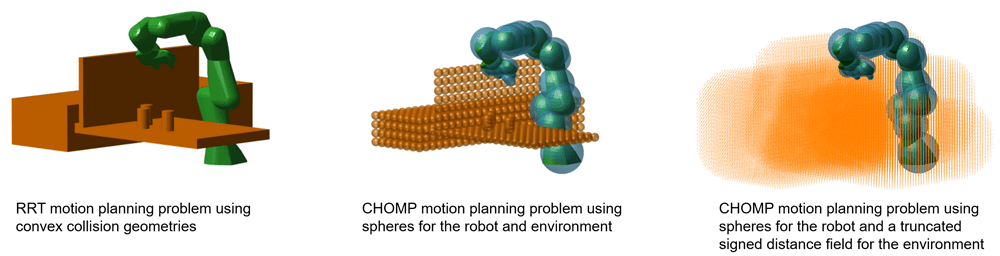
While planning a path using RRT, the planner queries only whether a waypoint is colliding or not. When planning a path using CHOMP, the algorithm requires the gradient of the collision cost of a waypoint. The gradient of the collision cost is the change in collision cost when there is a minor change in the waypoint. This means that you must model the environment as spheres for CHOMP, and as convex collision geometries for RRT.

This example shows you how to load a manipulator robot and a pick-and-place environment, model convex collision geometries as spherical obstacles for CHOMP, tune manipulatorCHOMP, and visualize the resulting pick-and-place trajectories.

Load Robot and Environment

Use the exampleHelperLoadPickAndPlaceCHOMP helper function to load a Franka Emika Panda manipulator robot model and slightly modify the gripper. The helper function also loads collision objects to act as the environment and returns a starting configuration. The starting conditions and environment are similar to the setup found in the Pick and Place Using RRT for Manipulators example.

[franka,startConfig,env] = exampleHelperLoadPickAndPlaceCHOMP;
indexOfCollisionObjectInEnvironmentToPick=3;

Create Environment and Robot Collision Model

While the environment env is ready for use with an RRT motion planner, CHOMP has stricter collision model representations:

The robot must be represented as a collection of spheres
The environment must be represented as a collection of spheres or as a signed distance field -- a discretized collision model of a set of meshes. For basic collision representation with spheres, only Robotics System Toolbox is required, but for the signed distance field, Navigation Toolbox is required.

This figure shows the difference in setup between using RRT and using CHOMP in the three possible permutations. Notice the overlaid spherical approximations, which CHOMP uses for collision costs, over the collision geometries of the robot.

Choose an Environment Representation

The sections below describe the different approaches to model the environment that are compatible with manipulatorCHOMP. There are two choices:

Collection of spheres: Model the environment as a collection of spheres that represent the volume of space occupied by the environment geometry.
Truncated signed distance field: Model the environment using MeshTSDF object, which allows users to pass collision geometries directly to CHOMP as inputs to the meshTSDF object, so there is no need to convert to spheres. Note that this requires Navigation Toolbox™.

In general, the meshTSDF representation is faster and may be simpler than recreating the environment as spheres. Both mechanisms approximate the true environment, but in different ways: sphere geometries approximate the environment as spheres and then use an exact gradient to compute collision cost within CHOMP, while the truncated signed distance field accepts collision meshes as input but approximates the gradient for collision cost. Hence, in most situations meshTSDF will be more appropriate, but when the environment is well-approximated by spheres, spheres may be better.

Model the Environment Using a Collection of Spheres

In this example, env is a cell array of collision geometries, represented as collisionBox and collisionCylinder objects. To ensure the optimization routine accounts for the collision geometries, create an array, sphobstacles, in which to store the approximated environment.

sphobstacles = [];

The objective of this example is to pick the third object in the env cell array, a soda can, and place it over the barricade on the other side of the platform. This process physically moves the soda can from one place to another. From the perspective of a motion planning problem, you must remove the spheres that represent the soda can from the spherical obstacles and attach them to the gripper such that they become a part of the spheres on the rigid body tree. Create an array to track the spheres associated with the object to be picked via spheresOfObjectToPick, and another for tracking the indices of these spheres in the sphobstacles array, spheresOfObjectToPickIdx.

indexOfCollisionObjectInEnvironmentToPick = 3;
spheresOfObjectToPickIdx = [];
spheresOfObjectToPick = [];

The environment cell array consists of collision boxes that represent the platforms and barricades, and collision cylinders that represent the soda cans to be picked and placed. The exampleHelperApproximateCollisionCylinderSpheres and exampleHelperApproximateCollisionBoxSpheres helper functions approximate an array of spheres for the box and sphere collision geometry types, respectively.

To approximate the collision cylinders using spheres, for each collision cylinder in the environment, fit a collision capsule using the fitCollisionCapsule object function, and then generate spheres on the capsule using genspheres at a ratio of [0 0.5 1]. This ratio generates a sphere at the beginning, middle, and end of the capsule. To more closely approximate the capsule, you can add more uniformly sampled ratio points.
To approximate spheres on a collision box, use the meshgrid function. Define the grid over the length, height, and width of the box, and place a sphere at each grid point. Assume 20 spheres per unit length of the box. Increasing this density creates more spheres, which can more accurately model a box, but results in higher computation times when optimizing a trajectory.

sphPerUnit = 20; % Spheres per unit length of box
for i = 1:length(env)
    if(isa(env{i},"collisionCylinder"))
        ratio = [0 0.5 1];
        sph = exampleHelperApproximateCollisionCylinderSpheres(env{i},ratio);
    else
        rho = 1/sphPerUnit;
        sph = exampleHelperApproximateCollisionBoxSpheres(env{i},rho);
    end
    if(i == indexOfCollisionObjectInEnvironmentToPick)
        spheresOfObjectToPickIdx = size(sphobstacles,2)+(1:size(sph,2));
        spheresOfObjectToPick = sph;
    end
    sphobstacles = [sphobstacles sph];
end

Model the Environment Using a Truncated Signed Distance Field

A simpler way to model the environment is to use a signed distance field via the meshTSDF manager. The signed distance field accepts a set of meshes or primitives and converts it to a discrete representation that returns a vector measure of closeness to collision between an abritrary point in space and the signed distance field, i.e. the signed distance. CHOMP can use this signed distance in the collision-avoidance pieces of the cost function, thereby allowing a user to model relatively complex environments efficiently for use with CHOMP.

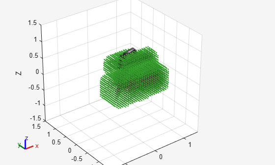
The following code shows how to model the environment with meshTSDF:

if exist('meshtsdf','class')
    meshStruct = geom2struct(env);
    manager=meshtsdf(meshStruct,"Resolution",15,"TruncationDistance",0.3);

    % Display visualization
    show(franka);
    hold all
    show(manager);
end

Create Planner Instance

Initialize both the picking and placing configurations. The picking configuration places the end effector of the robot over the desired soda can, and the placing configuration places the end effector on the other side of the barricade.

pickConfig = [0.2367 -0.0538 0.0536 -2.2101 0.0019 2.1565 -0.9682];
placeConfig = [-0.6564 0.2885 -0.3187 -1.5941 0.1103 1.8678 -0.2344];

Create a manipulatorCHOMP object from the robot rigid body tree, and set the SphericalObstacles property to the spherical approximation of the environment. Model the environment using the representation of choice. While these can be used together, in this example only one representation at a time is used. Note that the truncated signed distance field is an advanced collision representation and requires a Navigation Toolbox license.

envModelType="Signed Distance Field";
if envModelType=="Spherical Decomposition"
    chomp = manipulatorCHOMP(franka);
    chomp.SphericalObstacles = sphobstacles
    collisionsForVisuals = {}; % Don't display the original environment in the analysis visuals
else
    if ~exist('meshtsdf','class')
        error('The meshtsdf class requires a Navigation Toolbox License. Use Spherical Decomposition instead to run the example');
    end
    chomp = manipulatorCHOMP(franka, MeshTSDF=manager);
    collisionsForVisuals = env; % Display the original environment in the analysis visuals
end

For a collision-free trajectory, set a higher weight on the cost of collision as compared to smoothness. Increase the learning rate for higher convergence. Refer to the Tune Optimizer section to see the relationship between the various cost and solver options.

chomp.CollisionOptions.CollisionCostWeight = 10;
chomp.SmoothnessOptions.SmoothnessCostWeight = 1e-3;
chomp.SolverOptions.LearningRate = 5;

Visualize the starting, picking, and placing joint configurations of the robot for the CHOMP instance.

figure
show(chomp,[startConfig; pickConfig; placeConfig],CollisionObjects=collisionsForVisuals);
title("Starting, Picking, and Placing Configurations")
xlim([-1 1])
ylim([-1 1])
zlim([-0.2 1])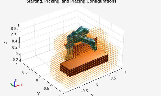

Compare Motion Planning Problems

Visualize the differences in the collision models for the environment and the robot between the CHOMP and RRT solvers.

subplot(1,2,1)
show(franka,startConfig,Collisions="on",Visuals="off");
hold on
for i = 1:length(env)
    show(env{i});
end
hold off
xlim([-1 1])
ylim([-1 1])
zlim([-0.2 1])
title("RRT Motion Planning Problem")

subplot(1,2,2)
show(chomp,startConfig,CollisionObjects=collisionsForVisuals);
xlim([-1 1])
ylim([-1 1])
zlim([-0.2 1])
title("CHOMP Motion Planning Problem")

Plan Picking Trajectory

Plan for an optimal collision-free picking trajectory. Assume a minimum-jerk trajectory between the starting and picking configurations. Additionally, assume the trajectory is 2 seconds long and is discretized in 0.1 second time steps.

[optimpickconfig,timestamppick,solpickinfo] = optimize(chomp,[startConfig; pickConfig], ... % Starting and ending robot joint configurations
                                                             [0 2], ...                    % Two waypoint times, first at 0s and last at 2s
                                                             0.10, ...                     % 0.1s time step
                                                             InitialTrajectoryFitType="minjerkpolytraj");

Display the IsCollisionFree and InitialCollisionCost fields of the solpickinfo structure, as well as the final collision cost of the CollisionCost field. Note that the IsCollisionFree field is true, meaning the trajectory is collision free, and the final collision cost of CollisionCost is lower than the initial collision cost. CHOMP is an optimization-based motion planner, so CHOMP treats the collisions during a trajectory as a cost and not a constraint. For more information on how CHOMP can output trajectories that result in collisions if you set weights inappropriately, see the Tune Optimizer section.

solpickinfo.IsCollisionFree

ans = logical
   1

solpickinfo.InitialCollisionCost

ans = 7.7603e-04

solpickinfo.CollisionCost(solpickinfo.Iterations)

ans = 3.0642e-04

solpickinfo.OptimizationTime

ans = 0.4357

Show the optimized configuration trajectory between the starting configuration and the picking configuration.

figure
show(chomp,optimpickconfig,CollisionObjects=collisionsForVisuals);
title("Optimized Picking Trajectory")
xlim([-1 1])
ylim([-1 1])
zlim([-0.2 1])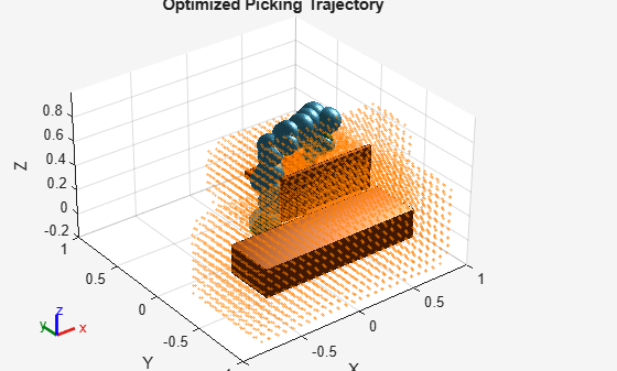

Plan Placing Trajectory

Remove the can as an obstacle in the CHOMP environment and get the transformation from the base of the robot to the hand of the robot. Then transform the spheres of the can so that they are in the end-effector frame, and add the spheres of the can to the cell array of spheres of the robot hand.

if envModelType=="Spherical Decomposition"
    chomp.SphericalObstacles(:,spheresOfObjectToPickIdx) = [];
else
    removeMesh(chomp.MeshTSDF, indexOfCollisionObjectInEnvironmentToPick);
end
Tee = getTransform(franka,pickConfig,"panda_hand");
spheresInEeFrame = transform(inv(se3(Tee)),spheresOfObjectToPick(2:end,:)')';
pandahandspheres = chomp.RigidBodyTreeSpheres("panda_hand","spheres").spheres{1};
chomp.RigidBodyTreeSpheres("panda_hand","spheres").spheres{1} = [pandahandspheres,[spheresOfObjectToPick(1,:);spheresInEeFrame]];

Plan the placing trajectory.

[optimplaceconfig,timestampplace,solplaceinfo] = optimize(chomp,[pickConfig; placeConfig], ...
                                                                [0 2], ...
                                                                0.10, ...
                                                                InitialTrajectoryFitType="minjerkpolytraj");

Note that the InitialCollisionCost is higher than the final collision cost, which is at or near zero.

solplaceinfo.InitialCollisionCost

ans = 0.6973

solplaceinfo.CollisionCost(solplaceinfo.Iterations)

ans = 8.2528e-04

Check the Collision-Free property, which indicates whether the collision cost has reached zero. Note that for the MeshTSDF environment model, the overall collision cost is near zero, but the status returns not collision-free. This is because of collisions perceived between spherical collision geometries that cause a fractional cost increase. The overall collision-free status can be verified via visualization.

solplaceinfo.IsCollisionFree

ans = logical
   0

The Opimization time records the overall time to plan.

solplaceinfo.OptimizationTime

ans = 0.2139

Show the optimized configuration trajectory between the picking configuration and the placing configuration.

figure
show(chomp,optimplaceconfig,CollisionObjects=collisionsForVisuals);
title("Optimized Placing Trajectory")
xlim([-1 1])
ylim([-1 1])
zlim([-0.2 1])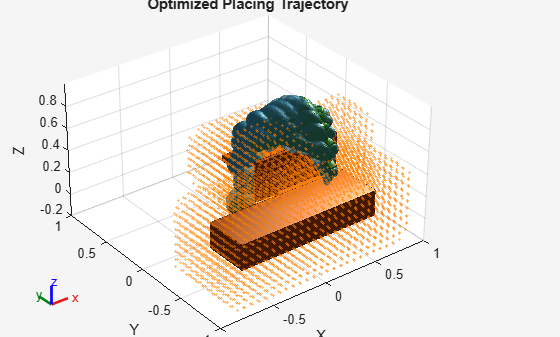

Tune Optimizer

CHOMP tries to find a balance between collision avoidance and smoothness a trajectory. The chompCollisionOptions, chompSmoothnessOptions, and chompSolverOptions objects help you specify how the solver should weigh these costs. These are the three parameters that you can tune to obtain an optimal trajectory:

CollisionCostWeight — A property of the chompCollisionOptions object, this value specifies how much weight the optimizer should place on the collision avoidance cost of the trajectory. This weight affects the rate of change of cost of collision of the trajectory per iteration. A higher value indicates a higher change per iteration in the collision cost.
SmoothnessCostWeight — A property of the chompSmoothnessOptions object, this value specifies how much weight the optimizer should place on smoothness of the trajectory. This weight affects the rate of change of the smoothness cost of the trajectory per iteration. A higher value indicates higher change per iteration in the smoothness cost.
LearningRate — A property of the chompSolverOptions object, this value specifies how the overall objective function, such as the sum of the weighted smoothness and collision costs, changes per iteration. A higher value indicates the trajectory updates faster per iteration.

Decrease Collision Cost Weight

Decrease the value of the CollisionCostWeight property and plan the placing trajectory again.

chomp.CollisionOptions.CollisionCostWeight = 1.5;
[placetraj,~,lowcollcostinfo] = optimize(chomp,[pickConfig; placeConfig], ...
                                               [0 2], ...
                                               0.10, ...
                                               InitialTrajectoryFitType="minjerkpolytraj");

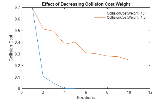
Plot the results of the planner with a collision cost weight of 10 and 1.5 to see the effect. Note that setting the collision cost weight to a lower value results in a higher collision cost when the optimizer completes its trajectory planning.

figure
plot([solplaceinfo.InitialCollisionCost,solplaceinfo.CollisionCost])
hold on
plot([lowcollcostinfo.InitialCollisionCost,lowcollcostinfo.CollisionCost])
title("Effect of Decreasing Collision Cost Weight")
legend({"CollisionCostWeight=10","CollisionCostWeight=1.5"})
xlabel("Iterations")
ylabel("Collision Cost")
hold off

Display the IsCollisionFree field of the solution info, and show the trajectory with this lower collision cost weight. Notice that the trajectory is not collision free after decreasing the collision cost weight to 1.5 and the final collision cost is significantly higher.

lowcollcostinfo.CollisionCost(lowcollcostinfo.Iterations)

ans = 0.2476

disp(lowcollcostinfo.IsCollisionFree)

show(chomp,placetraj,CollisionObjects=collisionsForVisuals);
xlim([-1 1])
ylim([-1 1])
zlim([-0.2 1])
title("Place Trajectory with CollisionCostWeight=1.5")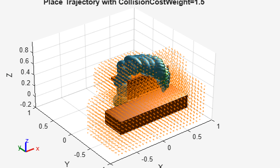

Increase Smoothness Cost Weight

Increase the smoothness cost weight to a value greater than the collision cost weight, indicating that smoothness is of a higher priority. Then, plan a place trajectory.

chomp.SmoothnessOptions.SmoothnessCostWeight = 0.1;
chomp.CollisionOptions.CollisionCostWeight = 1e-3;
[placetraj,~,highsmoothinfo] = optimize(chomp,[pickConfig; placeConfig], ...
                                            [0 2], ...
                                            0.10, ...
                                            InitialTrajectoryFitType="minjerkpolytraj");

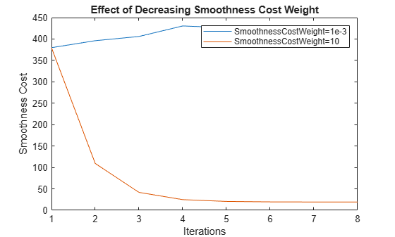
Plot the results for the smoothness cost weights of 1e-3 and 10 to see the effect. Note that setting the smoothness cost weight higher results in a higher collision cost when the optimizer completes its trajectory planning. When smoothness cost weight is lower, notice that the smoothness cost increases because the manipulator must take a longer path in the workspace to prioritize collision avoidance.

figure
plot([solplaceinfo.InitialSmoothnessCost,solplaceinfo.SmoothnessCost])
hold on
plot([highsmoothinfo.InitialSmoothnessCost,highsmoothinfo.SmoothnessCost])
title("Effect of Decreasing Smoothness Cost Weight")
legend({"SmoothnessCostWeight=1e-3","SmoothnessCostWeight=10"})
xlabel("Iterations")
ylabel("Smoothness Cost")
hold off

Display the IsCollisionFree field of the solution info and show the trajectory with the higher smoothness cost weight. Notice that the trajectory is not collision free after increasing the smoothness cost weight to 10 and the final collision cost is significantly higher.

highsmoothinfo.CollisionCost(highsmoothinfo.Iterations)

ans = 0.5689

disp(highsmoothinfo.IsCollisionFree)

show(chomp,placetraj,CollisionObjects=collisionsForVisuals);
title("Place Trajectory with SmoothnessCostWeight=1.5")
xlim([-1 1])
ylim([-1 1])
zlim([-0.2 1])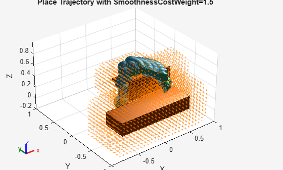

Decrease Learning Rate

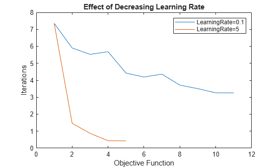
Decreasing the learning rate, while keeping the original smoothness and collision cost weights, results in the solver requiring more iterations for the solution to converge. Decrease the learning rate and return the collision and smoothness costs to their original values. Then, plan a place trajectory using the solver, and visualize the required iterations for the solver with the original learning rate and the decreased learning rate.

chomp.CollisionOptions.CollisionCostWeight = 10;
chomp.SmoothnessOptions.SmoothnessCostWeight = 1e-3;
chomp.SolverOptions.LearningRate = 0.5;
[placetraj,~,lowlearningrateinfo] = optimize(chomp,[pickConfig; placeConfig], ...
                                                   [0 2], ...
                                                   0.10, ...
                                                   InitialTrajectoryFitType="minjerkpolytraj");
figure
plot([lowlearningrateinfo.InitialObjectiveFunction,lowlearningrateinfo.ObjectiveFunction])
hold on
plot([solplaceinfo.InitialObjectiveFunction,solplaceinfo.ObjectiveFunction])
title("Effect of Decreasing Learning Rate")
legend({"LearningRate=0.1","LearningRate=5"})
xlabel("Objective Function")
ylabel("Iterations")

Visualize Trajectory

Visualize the picking and placing trajectories of the robot.

figure
subplot(1,2,1)
show(chomp,optimpickconfig,CollisionObjects=env);
xlim([-1 1])
ylim([-1 1])
zlim([-0.2 1])
view([pi 0 0])
title("Picking Trajectory")
subplot(1,2,2)
show(chomp,optimplaceconfig,CollisionObjects=env);
xlim([-1 1])
ylim([-1 1])
zlim([-0.2 1])
title("Placing Trajectory")
view([pi 0 0])

Visualize Robot Motion

Animate the trajectory of the robot for the entire pick-and-place task.

figure
show(franka,startConfig,Collisions="on",Visuals="off");
title("Animated Pick-and-Place Trajectory")
xlim([-1 1])
ylim([-1 1])
zlim([-0.2 1])
rc = rateControl(5);
view([pi 0 0])
hold on
for i = 1:length(env)
    if i == indexOfCollisionObjectInEnvironmentToPick
        [~,p] = show(env{i}); % Store patch of initial soda can location
    else
        show(env{i});
    end
end
exampleHelperVisualizePickTrajectory(franka,optimpickconfig,rc);
exampleHelperVisualizePlaceTrajectory(franka,env{indexOfCollisionObjectInEnvironmentToPick},optimplaceconfig,rc,p);
hold off