Main Content

nlmpcmove

Compute optimal control action for nonlinear MPC controller

Description

Nonlinear MPC

mv = nlmpcmove(nlobj,x,lastmv) computes the optimal control action for the current time. To simulate closed-loop nonlinear MPC control, call nlmpcmove repeatedly.

example

mv = nlmpcmove(nlobj,x,lastmv,ref) specifies reference values for the plant outputs. If you do not specify reference values, nlmpcmove uses zeros by default.

mv = nlmpcmove(nlobj,x,lastmv,ref,md) specifies run-time measured disturbance values. If your controller has measured disturbances, you must specify md.

example

mv = nlmpcmove(nlobj,x,lastmv,ref,md,options) specifies additional run-time options for computing optimal control moves. Using options, you can specify initial guesses for state and manipulated variable trajectories, update tuning weights at constraints, or modify prediction model parameters.

example

[mv,opt] = nlmpcmove(___) returns an nlmpcmoveopt object that contains initial guesses for the state and manipulated trajectories to be used in the next control interval.

example

[mv,opt,info] = nlmpcmove(___) returns additional solution details, including the final optimization cost function value and the optimal manipulated variable, state, and output trajectories.

Multistage Nonlinear MPC

example

mv = nlmpcmove(msobj,x,lastmv) computes the optimal control action for the current time. To simulate closed-loop nonlinear MPC control, call nlmpcmove repeatedly.

mv = nlmpcmove(msobj,x,lastmv,simdata) specifies the additional simdata structure, which contains measured disturbances, run-time bounds, parameters for the state and stage functions, and initial guesses for state and manipulated variable trajectories. In general use the following syntax to return a new simdata (containing updated initial guesses) as a second output argument.

[mv,simdata] = nlmpcmove(___) returns an updated simdata structure that contains new initial guesses for the state and manipulated trajectories to be used in the next control interval. Good initial guesses are important since they help the solver to converge to a solution faster.

[mv,simdata,info] = nlmpcmove(___) returns additional solution details, including the final optimization cost function value and the optimal manipulated variable, state, and output trajectories.

Examples

collapse all

Create a nonlinear MPC controller with six states, six outputs, and four inputs.

nx = 6;
ny = 6;
nu = 4;
nlobj = nlmpc(nx,ny,nu);
Zero weights are applied to one or more OVs because there are fewer MVs than OVs.

Specify the controller sample time and horizons.

Ts = 0.4;
p = 30;
c = 4;
nlobj.Ts = Ts;
nlobj.PredictionHorizon = p;
nlobj.ControlHorizon = c;

Specify the prediction model state function and the Jacobian of the state function. For this example, use a model of a flying robot.

nlobj.Model.StateFcn = "FlyingRobotStateFcn";
nlobj.Jacobian.StateFcn = "FlyingRobotStateJacobianFcn";

Specify a custom cost function for the controller that replaces the standard cost function.

nlobj.Optimization.CustomCostFcn = @(X,U,e,data) Ts*sum(sum(U(1:p,:)));
nlobj.Optimization.ReplaceStandardCost = true;

Specify a custom constraint function for the controller.

nlobj.Optimization.CustomEqConFcn = @(X,U,data) X(end,:)';

Specify linear constraints on the manipulated variables.

for ct = 1:nu
    nlobj.MV(ct).Min = 0;
    nlobj.MV(ct).Max = 1;
end

Validate the prediction model and custom functions at the initial states (x0) and initial inputs (u0) of the robot.

x0 = [-10;-10;pi/2;0;0;0];
u0 = zeros(nu,1); 
validateFcns(nlobj,x0,u0);
Model.StateFcn is OK.
Jacobian.StateFcn is OK.
No output function specified. Assuming "y = x" in the prediction model.
Optimization.CustomCostFcn is OK.
Optimization.CustomEqConFcn is OK.
Analysis of user-provided model, cost, and constraint functions complete.

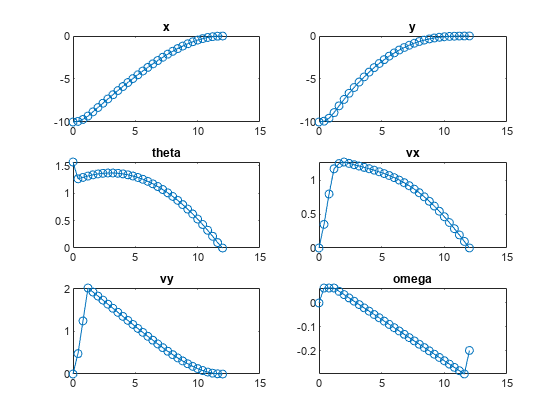
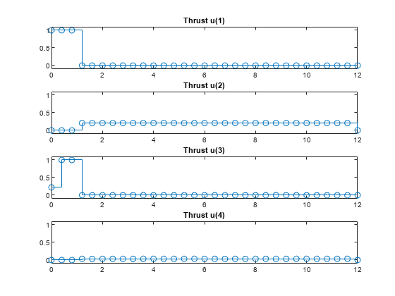
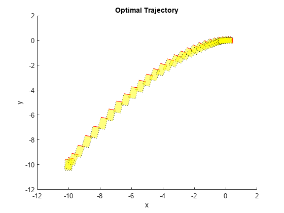
Compute the optimal state and manipulated variable trajectories, which are returned in the info.

[~,~,info] = nlmpcmove(nlobj,x0,u0);
Slack variable unused or zero-weighted in your custom cost function.
All constraints will be hard.

Plot the optimal trajectories.

FlyingRobotPlotPlanning(info,Ts)
Optimal fuel consumption =   1.884953

Create a nonlinear MPC controller with four states, two outputs, and one input.

nlobj = nlmpc(4,2,1);
Zero weights are applied to one or more OVs because there are fewer MVs than OVs.

Specify the sample time and horizons of the controller.

Ts = 0.1;
nlobj.Ts = Ts;
nlobj.PredictionHorizon = 10;
nlobj.ControlHorizon = 5;

Specify the state function for the controller, which is in the file pendulumDT0.m. This discrete-time model integrates the continuous time model defined in pendulumCT0.m using a multistep forward Euler method.

nlobj.Model.StateFcn = "pendulumDT0";
nlobj.Model.IsContinuousTime = false;

The prediction model uses an optional parameter, Ts, to represent the sample time. Specify the number of parameters.

nlobj.Model.NumberOfParameters = 1;

Specify the output function of the model, passing the sample time parameter as an input argument.

nlobj.Model.OutputFcn = @(x,u,Ts) [x(1); x(3)];

Define standard constraints for the controller.

nlobj.Weights.OutputVariables = [3 3];
nlobj.Weights.ManipulatedVariablesRate = 0.1;
nlobj.OV(1).Min = -10;
nlobj.OV(1).Max = 10;
nlobj.MV.Min = -100;
nlobj.MV.Max = 100;

Validate the prediction model functions.

x0 = [0.1;0.2;-pi/2;0.3];
u0 = 0.4;
validateFcns(nlobj, x0, u0, [], {Ts});
Model.StateFcn is OK.
Model.OutputFcn is OK.
Analysis of user-provided model, cost, and constraint functions complete.

Only two of the plant states are measurable. Therefore, create an extended Kalman filter for estimating the four plant states. Its state transition function is defined in pendulumStateFcn.m and its measurement function is defined in pendulumMeasurementFcn.m.

EKF = extendedKalmanFilter(@pendulumStateFcn,@pendulumMeasurementFcn);

Define initial conditions for the simulation, initialize the extended Kalman filter state, and specify a zero initial manipulated variable value.

x = [0;0;-pi;0];
y = [x(1);x(3)];
EKF.State = x;
mv = 0;

Specify the output reference value.

yref = [0 0];

Create an nlmpcmoveopt object, and specify the sample time parameter.

nloptions = nlmpcmoveopt;
nloptions.Parameters = {Ts};

Run the simulation for 10 seconds. During each control interval:

  1. Correct the previous prediction using the current measurement.

  2. Compute optimal control moves using nlmpcmove. This function returns the computed optimal sequences in nloptions. Passing the updated options object to nlmpcmove in the next control interval provides initial guesses for the optimal sequences.

  3. Predict the model states.

  4. Apply the first computed optimal control move to the plant, updating the plant states.

  5. Generate sensor data with white noise.

  6. Save the plant states.

Duration = 10;
xHistory = x;
for ct = 1:(Duration/Ts)
    % Correct previous prediction
    xk = correct(EKF,y);
    % Compute optimal control moves
    [mv,nloptions] = nlmpcmove(nlobj,xk,mv,yref,[],nloptions);
    % Predict prediction model states for the next iteration
    predict(EKF,[mv; Ts]);
    % Implement first optimal control move
    x = pendulumDT0(x,mv,Ts);
    % Generate sensor data
    y = x([1 3]) + randn(2,1)*0.01;
    % Save plant states
    xHistory = [xHistory x];
end

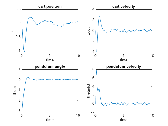
Plot the resulting state trajectories.

figure
subplot(2,2,1)
plot(0:Ts:Duration,xHistory(1,:))
xlabel('time')
ylabel('z')
title('cart position')
subplot(2,2,2)
plot(0:Ts:Duration,xHistory(2,:))
xlabel('time')
ylabel('zdot')
title('cart velocity')
subplot(2,2,3)
plot(0:Ts:Duration,xHistory(3,:))
xlabel('time')
ylabel('theta')
title('pendulum angle')
subplot(2,2,4)
plot(0:Ts:Duration,xHistory(4,:))
xlabel('time')
ylabel('thetadot')
title('pendulum velocity')

This example shows how to create and simulate a simple multistage MPC controller in closed loop, without using initial guesses, with the MATLAB® function nlmpcmove.

Create Multistage MPC Controller

Create a multistage nonlinear MPC object with a five-step horizon, one state, and one manipulated variable.

msobj = nlmpcMultistage(5,1,1);

Write a simple state function as a string.

sstr = "function xdot = mystatefcn(x,u)" + newline + ...
       "xdot = u-sin(x);" + newline + "end";

Write the string to the mystatefcn.m file.

sfid=fopen("mystatefcn.m","w");
fwrite(sfid,sstr,"char");
fclose(sfid);

Write a simple cost function as a string.

cstr = "function c = mycostfcn(k,x,u)" + newline + ...
       "c = abs(u)/k+k*x^2;" + newline + "end";

Write the string to the mycostfcn.m file.

cfid=fopen("mycostfcn.m","w");
fwrite(cfid,cstr,"char");
fclose(cfid);

Alternatively, you can write your state and cost MATLAB functions in the current folder (which is recommended because local functions are not supported for the generation of deployment code).

If files have not yet been written to the hard disk pause five second before accessing them.

if ~exist("mystatefcn","file")
    pause(5)
end

Specify the state transition function for the prediction model.

msobj.Model.StateFcn = "mystatefcn";

Specify the cost functions for last three stages.

for i=3:6
    msobj.Stages(i).CostFcn = "mycostfcn";
end

Note that, because the Jacobian of the state function is not supplied here, nlmpcmove needs to numerically calculate them at each time step, which negatively affects performance. As a best practice, supply the Jacobian of the state function, as shown in Simulate Multistage Nonlinear MPC Controller Using Initial Guesses. You can also automatically generate a Jacobian function using generateJacobianFunction.

Simulate Controller in Closed Loop

Initialize the plant state and input.

x=3;
mv=0;

Validate functions.

validateFcns(msobj,x,mv);
Model.StateFcn is OK.
"CostFcn" of the following stages [3 4 5 6] are OK.
Analysis of user-provided model, cost, and constraint functions complete.

Simulate the control loop for 5 steps, without updating the initial guess. Use the Euler method, that is dx(t)/dt ~ (x(t+1)-x(t))/Ts, to simulate the plant.

for k=1:5
    mv = nlmpcmove(msobj, x, mv);  % calculate move (without initial guess)
    x=x+0.2*mystatefcn(x,mv);      % update plant state assuming Ts=0.2s
end

Note that, because initial guesses are not supplied as an input argument, nlmpcmove needs to recalculate them at each time step, which negatively affects performance. Not supplying initial guesses can be an acceptable starting point, but in general is not suggested. As a best practice, use updated initial guesses at each time step, as shown in Simulate Multistage Nonlinear MPC Controller Using Initial Guesses, so that nlmpcmove does not need to recalculate them at each time step (in the same example you also use ode45 to calculate the evolution of the plant state until the next control interval).

Display the final values of the state and manipulated variables.

disp(['Final value of x =' num2str(x)])
Final value of x =1.3074
disp(['Final value of mv =' num2str(mv)])
Final value of mv =-0.35102

This example shows how to create and simulate a simple multistage MPC controller in closed loop using initial guesses, with the MATLAB® function nlmpcmove.

Create Multistage MPC Controller

Create a multistage MPC object with a seven-steps horizon, one state, and one manipulated variable.

msobj = nlmpcMultistage(7,1,1);

Defining your state and cost functions as separate files in the current folder on in a folder on the MATLAB path is recommended, as local functions are not supported for the generation of C/C++ deployment code. However, for this example, the state, cost, and state Jacobian functions are defined as local functions at the end of the example.

Specify the state transition function for the prediction model.

msobj.Model.StateFcn = @mystatefcn;

As a best practice, use Jacobians whenever they are available, otherwise the solver must compute it numerically. You can also automatically generate a Jacobian function using generateJacobianFunction.

Specify the Jacobian of the state transition function.

msobj.Model.StateJacFcn = @mystatejac;

Specify the cost functions for all stages except the first

for i=2:8
    msobj.Stages(i).CostFcn = @mycostfcn;
end

Define Initial Conditions, Create Data Structure, and Validate Functions

Initialize the plant state and input.

x=3;
mv=0;

Create the initial simulation data structure.

simdata = getSimulationData(msobj)
simdata = struct with fields:
    InitialGuess: []

Validate functions and the data structure.

validateFcns(msobj,x,mv,simdata);
Model.StateFcn is OK.
Model.StateJacFcn is OK.
"CostFcn" of the following stages [2 3 4 5 6 7 8] are OK.
Analysis of user-provided model, cost, and constraint functions complete.

Simulate Controller in Closed Loop

Simulate the control loop for 5 steps.

for k=1:5
    [mv,simdata] = nlmpcmove(msobj, x, mv, simdata);                  % calculate move and update simdata 
    [~,xhist] = ode45(@(t,xode) mystatefcn(xode,mv),[0 msobj.Ts],x);  % simulate plant for one sample time
    x = xhist(end);                                                     % update plant state
end

Since updated initial guesses are supplied as an input argument within the simdata structure, nlmpcmove does not need to recalculate them at each time step, which saves computation time and improves performance. Updating initial guesses at every time step is a best practice.

Display the last values of the state and manipulated variables.

disp(['Final value of x =' num2str(x)])
Final value of x =-0.039868
disp(['Final value of mv =' num2str(mv)])
Final value of mv =-0.067044

Support Functions

State transition function.

function xdot = mystatefcn(x,u)
    xdot = u-sin(x);
end

Jacobian of the state transition function.

function [A,B] = mystatejac(x,~)
    A = -cos(x);
    B = 1;
end

Stage cost functions.

function j = mycostfcn(s,x,u)
    j = abs(u)/s+s*x^2; 
end

Input Arguments

collapse all

Nonlinear MPC controller, specified as an nlmpc object.

Multistage nonlinear MPC controller, specified as an nlmpcMultistage object.

Current prediction model states, specified as a vector of lengthNx, where Nx is the number of prediction model states. Since the nonlinear MPC controller does not perform state estimation, you must either measure or estimate the current prediction model states at each control interval. For more information on nonlinear MPC prediction models, see Specify Prediction Model for Nonlinear MPC.

Control signals used in plant at previous control interval, specified as a vector of lengthNmv, where Nmv is the number of manipulated variables.

Note

Specify lastmv as the manipulated variable signals applied to the plant in the previous control interval. Typically, these signals are the values generated by the controller, though this is not always the case. For example, if your controller is offline and running in tracking mode; that is, the controller output is not driving the plant, then feeding the actual control signal to last_mv can help achieve bumpless transfer when the controller is switched back online.

Plant output reference values, specified as a row vector of length Ny or an array with Ny columns, where Ny is the number of output variables. If you do not specify ref, the default reference values are zero.

To use the same reference values across the prediction horizon, specify a row vector.

To vary the reference values over the prediction horizon from time k+1 to time k+p, specify an array with up to p rows. Here, k is the current time and p is the prediction horizon. Each row contains the reference values for one prediction horizon step. If you specify fewer than p rows, the values in the final row are used for the remaining steps of the prediction horizon.

Measured disturbance values, specified as a row vector of length Nmd or an array with Nmd columns, where Nmd is the number of measured disturbances. If your controller has measured disturbances, you must specify md. If your controller has no measured disturbances, specify md as [].

To use the same disturbance values across the prediction horizon, specify a row vector.

To vary the disturbance values over the prediction horizon from time k to time k+p, specify an array with up to p+1 rows. Here, k is the current time and p is the prediction horizon. Each row contains the disturbance values for one prediction horizon step. If you specify fewer than p rows, the values in the final row are used for the remaining steps of the prediction horizon.

Run-time options, specified as an nlmpcmoveopt object. Using these options, you can:

  • Tune controller weights

  • Update linear constraints

  • Set manipulated variable targets

  • Specify prediction model parameters

  • Provide initial guesses for state and manipulated variable trajectories

These options apply to only the current nlmpcmove time instant.

To improve solver efficiency, it is best practice to specify initial guesses for the state and manipulated variable trajectories.

Run-time simulation data, specified as structure. It must be initially created by getSimulationData, and then populated (if needed) before being passed to nlmpcmove as an input argument. An updated version is then always returned as a second output argument of nlmpcmove. Note that the MVMin, MVMax, StateMin, StateMax, MVRateMin, MVRateMax fields are needed only if you want to change these bounds at run time. These fields exist in the structure returned by getSimulationData only if you enable them explicitly when calling getSimulationData. The simdata structure has the following fields.

Measured disturbance values, specified as a row vector of length Nmd or an array with Nmd columns, where Nmd is the number of measured disturbances. If your multistage MPC object has any measured disturbance channel defined, you must specify MeasuredDisturbance. If your controller has no measured disturbances, this field does not exist in the structure generated by getSimulationData.

To use the same disturbance values across the prediction horizon, specify a row vector.

To vary the disturbance values over the prediction horizon from time k to time k+p, specify an array with up to p+1 rows. Here, k is the current time and p is the prediction horizon. Each row contains the disturbance values for one prediction horizon step. If you specify fewer than p rows, the values in the final row are used for the remaining steps of the prediction horizon.

Manipulated variable lower bounds, specified as a row vector of length Nmv or a matrix with Nmv columns, where Nmv is the number of manipulated variables. MVMin(:,i) replaces the ManipulatedVariables(i).Min property of the controller at run time.

To use the same bounds across the prediction horizon, specify a row vector.

To vary the bounds over the prediction horizon from time k to time k+p-1, specify a matrix with up to p rows. Here, k is the current time and p is the prediction horizon. Each row contains the bounds for one prediction horizon step. If you specify fewer than p rows, the final bounds are used for the remaining steps of the prediction horizon.

Manipulated variable upper bounds, specified as a row vector of length Nmv or a matrix with Nmv columns, where Nmv is the number of manipulated variables. MVMax(:,i) replaces the ManipulatedVariables(i).Max property of the controller at run time.

To use the same bounds across the prediction horizon, specify a row vector.

To vary the bounds over the prediction horizon from time k to time k+p-1, specify a matrix with up to p rows. Here, k is the current time and p is the prediction horizon. Each row contains the bounds for one prediction horizon step. If you specify fewer than p rows, the final bounds are used for the remaining steps of the prediction horizon.

Manipulated variable rate lower bounds, specified as a row vector of length Nmv or a matrix with Nmv columns, where Nmv is the number of manipulated variables. MVRateMin(:,i) replaces the ManipulatedVariables(i).RateMin property of the controller at run time. MVRateMin bounds must be nonpositive.

To use the same bounds across the prediction horizon, specify a row vector.

To vary the bounds over the prediction horizon from time k to time k+p-1, specify a matrix with up to p rows. Here, k is the current time and p is the prediction horizon. Each row contains the bounds for one prediction horizon step. If you specify fewer than p rows, the final bounds are used for the remaining steps of the prediction horizon.

Manipulated variable rate upper bounds, specified as a row vector of length Nmv or a matrix with Nmv columns, where Nmv is the number of manipulated variables. MVRateMax(:,i) replaces the ManipulatedVariables(i).RateMax property of the controller at run time. MVRateMax bounds must be nonnegative.

To use the same bounds across the prediction horizon, specify a row vector.

To vary the bounds over the prediction horizon from time k to time k+p-1, specify a matrix with up to p rows. Here, k is the current time and p is the prediction horizon. Each row contains the bounds for one prediction horizon step. If you specify fewer than p rows, the final bounds are used for the remaining steps of the prediction horizon.

State lower bounds, specified as a row vector of length Nx or a matrix with Nx columns, where Nx is the number of states. StateMin(:,i) replaces the States(i).Min property of the controller at run time.

To use the same bounds across the prediction horizon, specify a row vector.

To vary the bounds over the prediction horizon from time k+1 to time k+p, specify a matrix with up to p rows. Here, k is the current time and p is the prediction horizon. Each row contains the bounds for one prediction horizon step. If you specify fewer than p rows, the final bounds are used for the remaining steps of the prediction horizon.

State upper bounds, specified as a row vector of length Nx or a matrix with Nx columns, where Nx is the number of states. StateMax(:,i) replaces the States(i).Max property of the controller at run time.

To use the same bounds across the prediction horizon, specify a row vector.

To vary the bounds over the prediction horizon from time k+1 to time k+p, specify a matrix with up to p rows. Here, k is the current time and p is the prediction horizon. Each row contains the bounds for one prediction horizon step. If you specify fewer than p rows, the final bounds are used for the remaining steps of the prediction horizon.

State function parameter values, specified as a vector with length equal to the value of the Model.ParameterLength property of the multistage controller object. If Model.StateFcn needs a parameter vector, you must provide its value at runtime using this field. If Model.ParameterLength is 0 this field does not exist in the structure returned by getSimulationData.

Stage functions parameter values, specified as a vector with length equal to the sum of all the values in the Stages(i).ParameterLength properties of the multistage controller object. If any cost or constraint function defined in the Stages property needs a parameter vector, you must provide all the parameter vectors at runtime (stacked in a single column) using this field. If none of your stage functions have parameters, this field does not exist in the structure returned by getSimulationData.

You must stack the parameter vectors for all stages in the column vector StateFcnParameters as follows.

[parameter vector for stage 1;
 parameter vector for stage 2;
 ...
 parameter vector for stage p+1;
]

Terminal state, specified as a column vector with as many elements as the number of states. The terminal state is the desired state at the last prediction step. To specify desired terminal states at run-time via this field, you must specify finite values in the TerminalState field of the Model property of msobj. Specify inf for the states that do not need to be constrained to a terminal value. At run time, nlmpcmove ignores any values in the TerminalState field of simdata that correspond to inf values in msobj. If you do not specify any terminal value condition in msobj, this field is not created in simdata.

If there is no TerminalState in simdata then the terminal state constraint (if present) does not change at run time.

Initial guesses for the decision variables, specified as a column vector of length equal to the sum of the lengths of all the decision variable vectors for each stage. Good initial guesses are important since they help the solver to converge to a solution faster. Therefore, when simulating a control loop by calling nlmpcmove repeatedly in a loop, pass simdata as an input argument (so initial guesses can be used), and at the same time return an updated version of simdata (with new initial guesses for the next control interval) as an output argument.

You must be stack the initial guesses for all stages in the column vector InitialGuess as follows.

[state vector guess for stage 1;
 manipulated variable vector guess for stage 1;
 manipulated variable vector rate guess for stage 1; % if used
 slack variable vector guess for stage 1; % if used
 state vector guess for stage 2;
 manipulated variable vector guess for stage 2;
 manipulated variable vector rate guess for stage 2; % if used
 slack variable vector guess for stage 2; % if used
 ...
 state vector guess for stage p;
 manipulated variable vector guess for stage p;
 manipulated variable vector rate guess for stage p; % if used
 slack variable vector guess for stage p; % if used
 state vector guess for stage p+1;
 slack variable vector guess for stage p+1; % if used
]

If InitialGuess is [], the default initial guesses are calculated from the x and lastmv arguments passed to nlmpcmove.

In general, during closed-loop simulation, you do not specify InitialGuess yourself. Instead, when calling nlmpcmove, return the simdata output argument, which contains the calculated initial guesses for the next control interval. You can then pass simdata as an input argument to nlmpcmove for the next control interval. These steps are a best practice, even if you do not specify any other run-time options.

Output Arguments

collapse all

Optimal manipulated variable control action, returned as a column vector of length Nmv, where Nmv is the number of manipulated variables.

If the solver converges to a local optimum solution (info.ExitFlag is positive), then mv contains the optimal solution.

If the solver reaches the maximum number of iterations without finding an optimal solution (info.ExitFlag = 0) and:

  • nlobj.Optimization.UseSuboptimalSolution is true, then mv contains the suboptimal solution

  • nlobj.Optimization.UseSuboptimalSolution is false, then mv contains lastmv

If the solver fails (info.ExitFlag is negative), then mv contains lastmv.

Run-time options with initial guesses for the state and manipulated variable trajectories to be used in the next control interval, returned as an nlmpcmoveopt object. Any run-time options that you specified using options, such as weights, constraints, or parameters, are copied to opt.

The initial guesses for the states (opt.X0) and manipulated variables (opt.MV0) are the optimal trajectories computed by nlmpcmove and correspond to the last p-1 rows of info.Xopt and info.MVopt, respectively.

To use these initial guesses in the next control interval, specify opt as the options input argument to nlmpcmove.

Solution details, returned as a structure with the following fields.

Optimal manipulated variable sequence, returned as a (p+1)-by-Nmv array, where p is the prediction horizon and Nmv is the number of manipulated variables.

MVopt(i,:) contains the calculated optimal manipulated variable values at time k+i-1, for i = 1,...,p, where k is the current time. MVopt(1,:) contains the same manipulated variable values as output argument mv. Since the controller does not calculate optimal control moves at time k+p, MVopt(p+1,:) is equal to MVopt(p,:).

Optimal prediction model state sequence, returned as a (p+1)-by-Nx array, where p is the prediction horizon and Nx is the number of states in the prediction model.

Xopt(i,:) contains the calculated state values at time k+i-1, for i = 2,...,p+1, where k is the current time. Xopt(1,:) is the same as the current states in x.

Optimal output variable sequence, returned as a (p+1)-by-Ny array, where p is the prediction horizon and Ny is the number of outputs.

Yopt(i,:) contains the calculated output values at time k+i-1, for i = 2,...,p+1, where k is the current time. Yopt(1,:) is computed based on the current states in x and the current measured disturbances in md, if any.

Prediction horizon time sequence, returned as a column vector of length p+1, where p is the prediction horizon. Topt contains the time sequence from time k to time k+p, where k is the current time.

Topt(1) = 0 represents the current time. Subsequent time steps Topt(i) are Ts*(i-1), where Ts is the controller sample time.

Use Topt when plotting the MVopt, Xopt, or Yopt sequences.

Stacked slack variables vector, used in constraint softening. If all elements are zero, then all soft constraints are satisfied over the entire prediction horizon. If any element is greater than zero, then at least one soft constraint is violated.

The slack variable vector for all stages are stacked as:

[slack variable vector for stage 1; % if used
 slack variable vector for stage 2; % if used
 ...
 slack variable vector for stage p+1; % if used
]

Optimization exit code, returned as one of the following:

  • Positive Integer — Optimal solution found

  • 0 — Feasible suboptimal solution found after the maximum number of iterations

  • Negative integer — No feasible solution found

Number of iterations used by the nonlinear programming solver, returned as a positive integer.

Objective function cost, returned as a nonnegative scalar value. The cost quantifies the degree to which the controller has achieved its objectives.

The cost value is only meaningful when ExitFlag is nonnegative.

Updated run-time simulation data, returned as a structure, containing new initial guesses for the state and manipulated trajectories to be used in the next control interval. It is a structure with the following fields.

Measured disturbance values, specified as a row vector of length Nmd or an array with Nmd columns, where Nmd is the number of measured disturbances. If your multistage MPC object has any measured disturbance channel defined, you must specify MeasuredDisturbance. If your controller has no measured disturbances, this field does not exist in the structure generated by getSimulationData.

To use the same disturbance values across the prediction horizon, specify a row vector.

To vary the disturbance values over the prediction horizon from time k to time k+p, specify an array with up to p+1 rows. Here, k is the current time and p is the prediction horizon. Each row contains the disturbance values for one prediction horizon step. If you specify fewer than p rows, the values in the final row are used for the remaining steps of the prediction horizon.

Manipulated variable lower bounds, specified as a row vector of length Nmv or a matrix with Nmv columns, where Nmv is the number of manipulated variables. MVMin(:,i) replaces the ManipulatedVariables(i).Min property of the controller at run time.

To use the same bounds across the prediction horizon, specify a row vector.

To vary the bounds over the prediction horizon from time k to time k+p-1, specify a matrix with up to p rows. Here, k is the current time and p is the prediction horizon. Each row contains the bounds for one prediction horizon step. If you specify fewer than p rows, the final bounds are used for the remaining steps of the prediction horizon.

Manipulated variable upper bounds, specified as a row vector of length Nmv or a matrix with Nmv columns, where Nmv is the number of manipulated variables. MVMax(:,i) replaces the ManipulatedVariables(i).Max property of the controller at run time.

To use the same bounds across the prediction horizon, specify a row vector.

To vary the bounds over the prediction horizon from time k to time k+p-1, specify a matrix with up to p rows. Here, k is the current time and p is the prediction horizon. Each row contains the bounds for one prediction horizon step. If you specify fewer than p rows, the final bounds are used for the remaining steps of the prediction horizon.

Manipulated variable rate lower bounds, specified as a row vector of length Nmv or a matrix with Nmv columns, where Nmv is the number of manipulated variables. MVRateMin(:,i) replaces the ManipulatedVariables(i).RateMin property of the controller at run time. MVRateMin bounds must be nonpositive.

To use the same bounds across the prediction horizon, specify a row vector.

To vary the bounds over the prediction horizon from time k to time k+p-1, specify a matrix with up to p rows. Here, k is the current time and p is the prediction horizon. Each row contains the bounds for one prediction horizon step. If you specify fewer than p rows, the final bounds are used for the remaining steps of the prediction horizon.

Manipulated variable rate upper bounds, specified as a row vector of length Nmv or a matrix with Nmv columns, where Nmv is the number of manipulated variables. MVRateMax(:,i) replaces the ManipulatedVariables(i).RateMax property of the controller at run time. MVRateMax bounds must be nonnegative.

To use the same bounds across the prediction horizon, specify a row vector.

To vary the bounds over the prediction horizon from time k to time k+p-1, specify a matrix with up to p rows. Here, k is the current time and p is the prediction horizon. Each row contains the bounds for one prediction horizon step. If you specify fewer than p rows, the final bounds are used for the remaining steps of the prediction horizon.

State lower bounds, specified as a row vector of length Nx or a matrix with Nx columns, where Nx is the number of states. StateMin(:,i) replaces the States(i).Min property of the controller at run time.

To use the same bounds across the prediction horizon, specify a row vector.

To vary the bounds over the prediction horizon from time k+1 to time k+p, specify a matrix with up to p rows. Here, k is the current time and p is the prediction horizon. Each row contains the bounds for one prediction horizon step. If you specify fewer than p rows, the final bounds are used for the remaining steps of the prediction horizon.

State upper bounds, specified as a row vector of length Nx or a matrix with Nx columns, where Nx is the number of states. StateMax(:,i) replaces the States(i).Max property of the controller at run time.

To use the same bounds across the prediction horizon, specify a row vector.

To vary the bounds over the prediction horizon from time k+1 to time k+p, specify a matrix with up to p rows. Here, k is the current time and p is the prediction horizon. Each row contains the bounds for one prediction horizon step. If you specify fewer than p rows, the final bounds are used for the remaining steps of the prediction horizon.

State function parameter values, specified as a vector with length equal to the value of the Model.ParameterLength property of the multistage controller object. If Model.StateFcn needs a parameter vector, you must provide its value at runtime using this field. If Model.ParameterLength is 0 this field does not exist in the structure returned by getSimulationData.

Stage functions parameter values, specified as a vector with length equal to the sum of all the values in the Stages(i).ParameterLength properties of the multistage controller object. If any cost or constraint function defined in the Stages property needs a parameter vector, you must provide all the parameter vectors at runtime (stacked in a single column) using this field. If none of your stage functions have parameters, this field does not exist in the structure returned by getSimulationData.

You must stack the parameter vectors for all stages in the column vector StateFcnParameters as follows.

[parameter vector for stage 1;
 parameter vector for stage 2;
 ...
 parameter vector for stage p+1;
]

Terminal state, specified as a column vector with as many elements as the number of states. The terminal state is the desired state at the last prediction step. To specify desired terminal states at run-time via this field, you must specify finite values in the TerminalState field of the Model property of msobj. Specify inf for the states that do not need to be constrained to a terminal value. At run time, nlmpcmove ignores any values in the TerminalState field of simdata that correspond to inf values in msobj. If you do not specify any terminal value condition in msobj, this field is not created in simdata.

If there is no TerminalState in simdata then the terminal state constraint (if present) does not change at run time.

Initial guesses for the decision variables, specified as a column vector of length equal to the sum of the lengths of all the decision variable vectors for each stage. Good initial guesses are important since they help the solver to converge to a solution faster. Therefore, when simulating a control loop by calling nlmpcmove repeatedly in a loop, pass simdata as an input argument (so initial guesses can be used), and at the same time return an updated version of simdata (with new initial guesses for the next control interval) as an output argument.

You must be stack the initial guesses for all stages in the column vector InitialGuess as follows.

[state vector guess for stage 1;
 manipulated variable vector guess for stage 1;
 manipulated variable vector rate guess for stage 1; % if used
 slack variable vector guess for stage 1; % if used
 state vector guess for stage 2;
 manipulated variable vector guess for stage 2;
 manipulated variable vector rate guess for stage 2; % if used
 slack variable vector guess for stage 2; % if used
 ...
 state vector guess for stage p;
 manipulated variable vector guess for stage p;
 manipulated variable vector rate guess for stage p; % if used
 slack variable vector guess for stage p; % if used
 state vector guess for stage p+1;
 slack variable vector guess for stage p+1; % if used
]

If InitialGuess is [], the default initial guesses are calculated from the x and lastmv arguments passed to nlmpcmove.

In general, during closed-loop simulation, you do not specify InitialGuess yourself. Instead, when calling nlmpcmove, return the simdata output argument, which contains the calculated initial guesses for the next control interval. You can then pass simdata as an input argument to nlmpcmove for the next control interval. These steps are a best practice, even if you do not specify any other run-time options.

Tips

During closed-loop simulations, it is best practice to warm start the nonlinear solver by using the predicted state and manipulated variable trajectories from the previous control interval as the initial guesses for the current control interval. To use these trajectories as initial guesses:

  1. Return the opt output argument when calling nlmpcmove. This nlmpcmoveopt object contains any run-time options you specified in the previous call to nlmpcmove, along with the initial guesses for the state (opt.X0) and manipulated variable (opt.MV0) trajectories.

  2. Pass this object in as the options input argument to nlmpcmove for the next control interval.

These steps are a best practice, even if you do not specify any other run-time options.

Version History

Introduced in R2018b