Field-Oriented Control of PMSM Using Position Estimated by Neural Network
This example shows how to implement field-oriented control (FOC) of a permanent magnet synchronous motor (PMSM) using a rotor position estimated by an autoregressive neural network (ARNN) trained with Deep Learning Toolbox™.
An FOC algorithm requires real-time rotor position feedback to implement speed control as well as to perform mathematical transformation on the reference stator voltages and feedback currents. Traditionally, such algorithms rely on physical sensors. However, due to increased accuracy and cost effectiveness, sensorless position estimation solutions can act as a better alternative to physical sensors.
The example provides one such sensorless solution that uses neural-network-based artificial intelligence (AI) to estimate real-time rotor position. You can use this example to train a neural network using data generated by an existing quadrature-encoder-sensor-based FOC algorithm. The trained neural network acts as a virtual position sensor and estimates the rotor position.
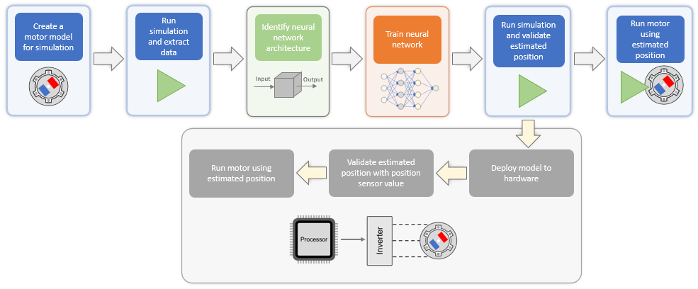
The example guides you through the workflow to train, simulate, and implement the neural network using the following steps:
Generate data needed to train the neural network.
Extract relevant data from the generated data.
Concatenate extracted data.
Process concatenated data.
Train the neural network using processed data.
Export the trained neural network to a Simulink® model associated with this example.
You can then simulate and deploy the Simulink model containing the trained neural network to the hardware and run a PMSM using FOC.
The following figure shows the entire workflow to implement a neural-network-based virtual position sensor.
Note:
This example enables you to use either the trained neural network or the quadrature encoder sensor to obtain the rotor position.
By default, the example guides you to generate the training data by simulating a model of the motor. However, if you have training data obtained from hardware running an actual motor, you can also use such a data set to train the neural network.
Model
The example uses the Simulink model mcb_pmsm_foc_qep_deep_learning_f28379d.
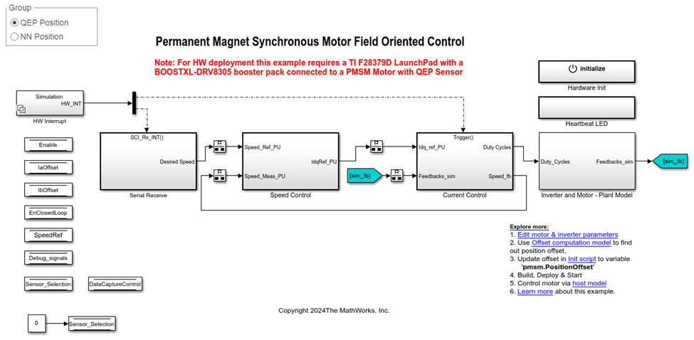
Using this model you can:
Generate the data needed to train the neural network.
Accommodate the trained neural network.
Run a PMSM using FOC in simulation or on hardware.
This model supports simulation and code generation.
Model Architecture
This figure shows the architecture of the FOC algorithm that the mcb_pmsm_foc_qep_deep_learning_f28379d model implements:
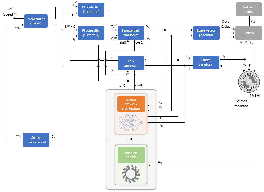
The model enables you to use a trained neural network or the quadrature encoder sensor to get the rotor position.
As shown in the figure, the neural network uses the Vα, Vβ, Iα, and Iβ inputs to output θe, sinθe, and cosθe, where:
Vα and Vβ are the voltages across the α and β axes, respectively (in per-unit).
Iα and Iβ are the currents across the α and β axes, respectively (in per-unit).
θe is the motor electrical position (in per-unit).
For more details about the per-unit (PU) system, see Per-Unit System.
You must train the neural network by using the Vα, Vβ, Iα, Iβ, and θe data so that it can accurately map the inputs into the output and act like a virtual position sensor by estimating the rotor position.
Generate Training Data from Target Simulink Model
The first step to using the example is to generate the Vα, Vβ, Iα, Iβ, and θe data needed to train the neural network. You can generate the data by using the TrainingDataCapture utility function. This function gets the training data by simulating the model mcb_pmsm_foc_qep_deep_learning_f28379d.slx, which contains a quadrature-encoder-sensor-based FOC algorithm. During simulation, the model performs a sweep across speed and torque reference values to capture the electrical position and the α- and β-equivalents of the stator voltages and currents.
What Is a Sweep Operation?
Using a sweep operation, the TrainingDataCapture utility function:
Selects a range of speed-torque operating points.
Simulates the model to run the quadrature-encoder-based FOC at each operating point (or a reference speed-torque value pair) for a limited time.
After the stator voltages and currents reach a steady state, records the resulting values of Vα, Vβ, Iα, Iβ, and θe.
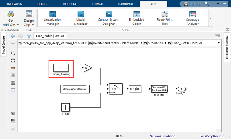
The following figures highlight the constant blocks that the utility function uses to select each operating point. The utility function uses:
Block Speed_Training(available in themcb_pmsm_foc_qep_deep_learning_f28379d/Serial Receive/SCI_Rx/Simulationsubsystem) to select a speed reference value.
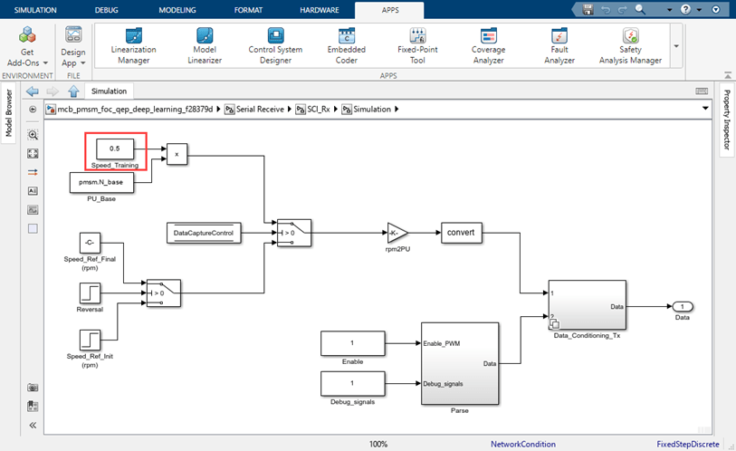
Block Torque_Training(available in themcb_pmsm_foc_qep_deep_learning_f28379d/Inverter and Motor - Plant Model/Simulation/Load_Profile (Torque)subsystem) to select a speed-torque operating point.
Subsystem
mcb_pmsm_foc_qep_deep_learning_f28379d/Current Control/Control_System/Closed Loop Control/Subsystemto capture the Vα, Vβ, Iα, Iβ, and θe values that correspond to the captured operating point and records them in aSimulink.SimulationOutputobject.
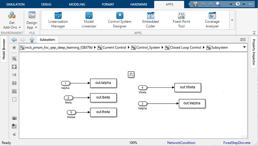
The TrainingDataCapture utility function also manually computes and records the sinθe and cosθe values for the captured operating point.
Speed Ranges for Sweep Operation
The TrainingDataCapture utility function performs the sweep operation by selecting operating points across these speed ranges:
Zero to low-speed range, which corresponds to 0% to 10% of the motor rated speed. In this range, the utility function minimizes sweep operations for the load torque. Because this speed range shows minimal load torque variations in real-world applications, the utility function keeps the training data lean in this speed range by maintaining an almost constant torque reference. The utility function primarily varies only speed references and collects only limited training data from this speed range.
Low to high-speed range, which corresponds to 10% to 100% of the motor rated speed. The utility function creates operating points by varying reference speed and torque values in this speed range to collect the majority of the required training data.
Duration of Capture for Each Operating Point
The TrainingDataCapture utility function simulates the target model at each speed-torque operating point. After simulation begins for an operating point, the utility function captures the Vα, Vβ, Iα, Iβ, and θe data for a limited duration defined by these variables:
Variables
dCStartTime1anddCEndTime1define the duration of data capture in the zero to low-speed range. Because of lower motor speeds, the duration of data capture is usually large in this range.Variables
dCStartTime2anddCEndTime2define the duration of data capture in the low to high-speed range. Because of higher motor speeds, the duration of data capture is usually small in this range.
With this approach, the utility function captures data only after the stator currents and voltages reach a steady state (after simulation begins).
You can tune these variables by modifying this live script.
Number of Reference Speed and Torque Data Capture Points
You can also use these variables to define the number of reference speed and torque data capture points.
Variable
dPSpdZtoLdefines the number of reference speed points that the utility function uses in the zero to low-speed range.Variable
dPSpdLtoHdefines the number of reference speed points that the utility function uses in the low to high-speed range.Variable
dPTorLtoHdefines the number of reference torque points that the utility function uses in the low to high-speed range.
Because the utility function uses a relatively fixed torque reference during the zero to low-speed range, the number of reference torque points is fixed in this range.
You can tune these variables by modifying this live script.
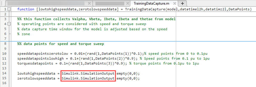
The utility function captures, appends, and stores the data for the operating points in the Simulink.SimulationOutput object, as this figure shows.
Run this code to generate the training data.
Note: Running the TrainingDataCapture utility function using these parameters can take approximately three hours.
%% Capture the training data using Simulink Environment
model='mcb_pmsm_foc_qep_deep_learning_f28379d';% Minor updates in model required for obtaining training data
dCStartTime1 = 3.8; %dataCaptureStartTime for low to high speed
dCEndTime1 = 4; %dataCaptureEndTime for low to high speed
dCStartTime2 = 3.5; %dataCaptureStartTime for zero to low speed
dCEndTime2 = 4; %dataCaptureEndTime for zero to low speed
dPSpdLtoH =40; %dataPointsSpeedLowtoHigh
dPSpdZtoL = 100;%dataPointsSpeedZerotoLow
dPTorLtoH =25; %data points torque (low(0.1pu) to high(1pu) speed)
[lowtohighspeeddata,zerotolowspeeddata] = ...
    TrainingDataCapture(model,[dCStartTime1,dCEndTime1],[dCStartTime2,dCEndTime2], ...
                        [dPSpdZtoL,dPSpdLtoH,dPTorLtoH]);
The TrainingDataCapture utility function stores the generated data in these Simulink.SimulationOutput objects:
Object
zerotolowspeeddatastores the data obtained by using the sweep operation across the zero to low-speed range.Object
lowtohighspeeddatastores the data obtained by using the sweep operation across the low to high-speed range.
To access the TrainingDataCapture utility function, click TrainingDataCapture.
Refine and Process Data
The next step is to extract the relevant data from the data that you generated in the previous section and then process it.
Extract One Electrical Cycle of Data
In the previous section, for each speed-torque operating point, the utility function TrainingDataCapture captured data for multiple electrical cycles during the time interval defined by the variables dCStartTime1, dCEndTime1, dCStartTime2, and dCEndTime2.
You can use the utility function OneElecCycleExtrac to refine the extracted data for each operating point by extracting one electrical cycle of data for each operating point.
Use these commands to extract one electrical cycle of data for each operating point captured in the Simulink.SimulationOutput objects lowtohighspeeddata and zerotolowspeeddata.
oneCycleDataLtoH = OneElecCycleExtrac(lowtohighspeeddata);
oneCycleDataZtoL = OneElecCycleExtrac(zerotolowspeeddata);
The utility function returns the refined data to these Simulink.SimulationOutput objects:
Object
oneCycleDataZtoLstores the electrical cycle of data for the zero to low-speed range.Object
oneCycleDataLtoHstores the electrical cycle of data for the low to high-speed range.
To access the OneElecCycleExtrac utility function, click OneElecCycleExtrac.
Concatenate One-Electrical-Cycle Data
Use the utility function DataConcatenate to concatenate the one-electrical-cycle data output.
Use this command to concatenate the extracted data stored in the Simulink.SimulationOutput objects oneCycleDataZtoL and oneCycleDataLtoH.
completeData = DataConcatenate(oneCycleDataLtoH,oneCycleDataZtoL);
The utility function returns the concatenated data to the Simulink.SimulationOutput object completeData.
To access the DataConcatenate utility function, click DataConcatenate.
Process Concatenated One-Electrical-Cycle Data
This example splits the data obtained after concatenation into these data sets:
Training data set, which includes 70% of data in the object
completeData. The example uses this data set to train the neural network.Validation data set, which includes the remaining 15% of data in the object
completeData. The example uses this data set to validate the trained neural network.Testing data set, which includes the next 15% of data in the object completeData. The example uses this data set to test the trained neural network.
Run this code to split the data in the object completeData:
tPLtoH=dPSpdLtoH*dPTorLtoH; % Total data points from speed and torque sweep in the low to high range
tPZtoH=(dPSpdLtoH*dPTorLtoH)+dPSpdZtoL; % Total data points from speed and torque sweep in the zero to high range
[traindatain,traindataout,testdatain,testdataout,validatedatain,validatedataout] ...
          = DataPreparation(completeData,tPLtoH,tPZtoH)
The utility function DataPreparation accepts these arguments:
Object
completeDataSimulink.SimulationOutput, which stores the output of theDataConcatenateutility functionVariable
tPLtoH, which corresponds todPSpdLtoHdPTorLtoHVariable
tPZtoH, whichcorresponds to (dPSpdLtoHdPTorLtoH) +dPSpdZtoL
The function returns the split data and stores it in these dlarray objects:
Object
traindatain, whichstores the portion of the training data set that the neural network uses as input.Object
traindataout, whichstores the portion of the training data set that the neural network uses as output.Object
testdatain, whichstores the portion of the testing data set that the neural network uses as input.Object
testdataout, whichstores the portion of the testing data set that the neural network uses as output.Object
validatedatain, whichstores the portion of the validation data set that the neural network uses as input.Object
validatedataout, whichstores the portion of the validation data set that the neural network uses as output.
To access the DataPreparation utility function, click DataPreparation.
Train and Test Neural Network
The next step is to select a neural network and train it by using the processed data that you generated in the previous section.
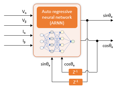
This example uses an autoregressive neural network (ARNN) and this series-parallel architecture:

In the figure:
Vα, Vβ, Iα, Iβ, , and are the true values of the time-series training data input.
and are the true values of the time-series training data input with a delay of one sample time.
and are the output predicted by the neural network.
The series-parallel architecture uses the Vα, Vβ, Iα, Iβ, , and input to predict the and output.
You can design and train this neural network by using either of these deep learning frameworks:
MATLAB Deep Learning Toolbox
PyTorch
Design and Train Neural Network in MATLAB
The Deep Learning Toolbox product provides functions, apps, and Simulink blocks for designing, implementing, and simulating deep neural networks. You use MATLAB code to design, train, and test your neural network. Then, you can export the network to Simulink for deployment to hardware.
The example provides you with the utility function CreateNetwork to train a neural network and build a nonlinear ARNN that can estimate rotor position. The utility function CreateNetwork uses the Deep Learning Toolbox object dlnetwork (Deep Learning Toolbox) and function trainnet (Deep Learning Toolbox) to create and train a neural network.
Use this code to train, test, and validate the neural network.
[posnet,testdatamse] = CreateNetwork(traindatain,traindataout,testdatain, ...
                                 testdataout,validatedatain,validatedataout)
The utility function CreateNetwork specifies the dlarray objects traindatain, traindataout, testdatain, testdataout, validatedatain, and validatedataout and returns the trained ARNN and the mean-square error information to this object and variable:
Object
posnet dlnetwork, which stores the trained ARNNVariable
testdatamse, which stores the mean squared error information that the utility function generated from the testing data set
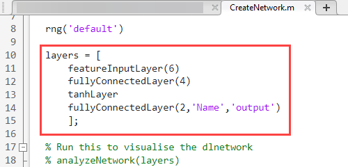
The CreateNetwork utility function generates a trained ARNN that contains two fully connected layers and an activation layer.
This figure shows the code that defines the neural network layers.
To access the CreateNetwork utility function, click CreateNetwork.
For more detail about the training process, see Building Neural Network for Virtual Position Sensing.
Design and Train Neural Network in PyTorch
If you prefer to work in other deep learning frameworks, such as PyTorch, you can use the Deep Learning Toolbox to import an existing neural network into MATLAB and deploy the network by using Simulink.
This example provides the PyTorch script createNetworkPy.py for training a neural network of the architecture described in Design and Train Neural Network in MATLAB. The script uses the same data that the MATLAB approach uses and captures the data in the dlnetwork object completeData.
In MATLAB, prepare the data for use in the PyTorch script:
prepareDataPy(completeData)
The PyTorch script createNetworkPy.py exports the trained neural network from PyTorch in the ONNX format, which facilitates importing the network into MATLAB.
In MATLAB, import the network.
posnet = importNetworkFromONNX("mlp_model.onnx","InputDataFormats","BC", ...
    "OutputDataFormates","BC")
The dlnetwork object that this command creates contains the same layers as the neural network designed by using the Deep Learning Toolbox and a custom output layer. The custom output layer is not needed. Remove that layer when you export the network to a Simulink model.
Export Trained Neural Network to Simulink Model
After you train the neural network, export the trained ARNN to a Simulink model by using the Deep Learning Toolbox function exportNetworkToSimulink. This function exports the trained ARNN network net to Simulink layer blocks that you can include in a model for simulation and code generation.
Export the trained ARNN net to Simulink layer blocks.
exportNetworkToSimulink(posnet)
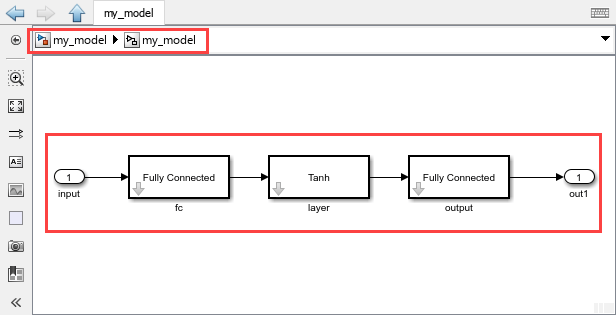
The exportNetworkToSimulink function uses the dlnetwork object net to create the Simulink layer blocks in a new Simulink model, as this figure shows.
If you export the dlnetwork object net that was created by importing a PyTorch neural network, the exportNetworkToSimulink function adds a placeholder subsystem outputOutput before the model output. Before using the layer blocks created during the export operation, replace the placeholder subsystem with a Reshape block, as this figure shows.
The Reshape block adjusts the dimensionality of the input signal to a dimensionality that you specify for the output.
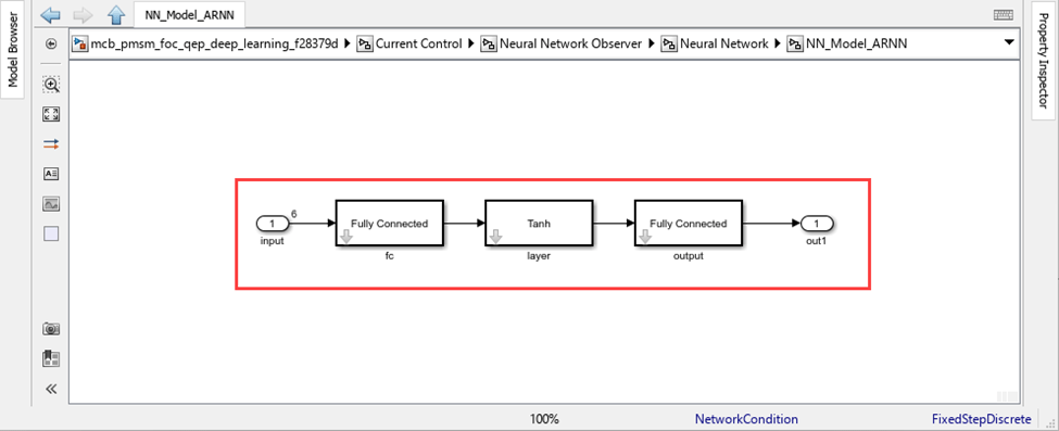
Copy the blocks that are in the generated model. Then, in the example model mcb_pmsm_foc_qep_deep_learning_f28379d.slx, paste the copied blocks in the subsystem mcb_pmsm_foc_qep_deep_learning_f28379d/Current Control/Neural Network Observer/Neural Network/NN_Model_ARNN.
These figures show the resulting architecture of the ARNN, which acts as a virtual position sensor. To achieve optimal performance with timeseries predictions, the example provides the previous output values (sinθe and cosθe) as additional inputs (with a delay).

Example model mcb_pmsm_foc_qep_deep_learning_f28379d.slx provides you with an option to switch between neural network-based and quadrature encoder-based position sensing.
Simulate and Deploy Code
After you export the neural network to Simulink, run this command to open the updated model.
open_system('mcb_pmsm_foc_qep_deep_learning_f28379d.slx');Simulate Target Model
1. In the target model mcb_pmsm_foc_qep_deep_learning_f28379d.slx, click one of these buttons:
QEP Position to use the quadrature encoder position sensor
NN Position to use the neural network that you trained using this example
2. Simulate the model. On the Simulation tab, click Run.
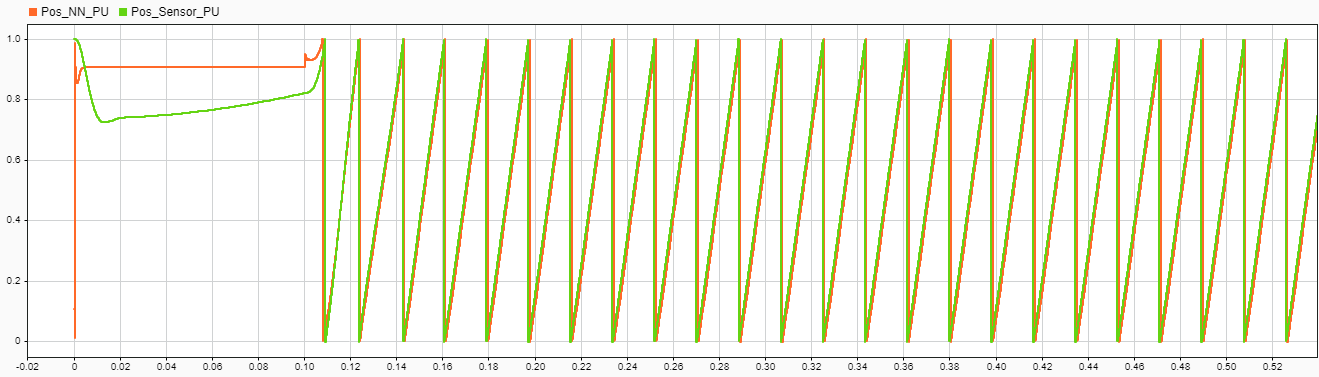
3. View and analyze the simulation results.On the Simulation tab, click Data Inspector.
This figure compares the position obtained by using the quadrature encoder sensor and the position estimated by the trained neural network.

Required Hardware
This example supports the LAUNCHXL-F28379D controller + BOOSTXL-DRV8305 inverter hardware configuration.
Generate and Deploy Code to Target Hardware
1. Simulate the target model and observe the simulation results.
2. Complete the hardware connections. For details about hardware connections related to the LAUNCHXL-F28379D controller + BOOSTXL-DRV8305 inverter hardware configuration, see LAUNCHXL-F28069M and LAUNCHXL-F28379D Configurations.
3. The model automatically computes the ADC (or current) offset values. To disable this functionality, which is enabled by default, in the model initialization script, change the value of the variable inverter.ADCOffsetCalibEnable to 0. Alternatively, in the model initialization script, you can compute the ADC offset values and update the variable setting manually. For instructions, see Run 3-Phase AC Motors in Open-Loop Control and Calibrate ADC Offset.
4. To use the trained neural network for position estimation, in the model, click the NN Position button.
5. To use the quadrature encoder sensor, in the model, click the QEP Position button. In addition, compute the encoder index offset value and update it in the model initialization script associated with the model. For instructions, see Quadrature Encoder Offset Calibration for PMSM.
6. Load a sample program, such as a program that operates the CPU2 blue LED, to CPU2 of LAUNCHXL-F28379D, by using GPIO31 (c28379D_cpu2_blink.slx). Doing so prevents CPU2 from being mistakenly configured to use the board peripherals intended for CPU1. For more information about the sample program or model, see the Task 2 - Create, Configure and Run the Model for TI Delfino F28379D LaunchPad (Dual Core) section in Getting Started with Texas Instruments C2000 Microcontroller Blockset (C2000 Microcontroller Blockset).
7. Deploy the target model to the hardware. On the Hardware tab, click Build, Deploy & Start.
8. Open the associated host model. In the model, click host model. For details about the serial communication between the host and target models, see Host-Target Communication.
9. In the model initialization script associated with the target model, specify the communication port by using the variable target.comport. The example uses this variable to update the Port parameter of the Host Serial Setup, Host Serial Receive, and Host Serial Transmit blocks available in the host model.
10. In the host model, update the Reference Speed (RPM) value.
11. Run the host model. On the Simulation tab, click Run.
12. Start running the motor by changing the position of the Start / Stop Motor switch to On.
13. Use the display and scope blocks available on the host model to monitor the debug signals.
See Also
analyzeNetwork (Deep Learning Toolbox) | fullyConnectedLayer (Deep Learning Toolbox) | tanhLayer (Deep Learning Toolbox) | dlnetwork (Deep Learning Toolbox) | trainnet (Deep Learning Toolbox)
Topics
- Field-Oriented Control of PMSM Using Position Estimated by Neural Network on STM32 Processor Based Boards (STM32 Microcontroller Blockset)
- Building Neural Network for Virtual Position Sensing
- List of Deep Learning Layers (Deep Learning Toolbox)