深層学習ワークフローのためのイメージの拡張

この例では、一般的な種類のランダムなイメージ拡張 (幾何学的変換、トリミング、ノイズの追加など) をどのように実行できるかを示します。

Image Processing Toolbox 関数により、一般的なスタイルのイメージ拡張の実装が可能になります。この例では、5 種類の一般的な変換を示します。

• ランダムなイメージ ワーピング変換

• トリミング変換

• 色変換

• 合成ノイズ

• 合成ぼかし

その後、この例では、複数の種類の変換を組み合わせて、データストア内のイメージ データに対する拡張の適用を実行する方法を示します。

拡張した学習データを使用してネットワークに学習させることができます。拡張したイメージを使用してネットワークに学習させる例については、image-to-image 回帰用のデータストアの準備 (Deep Learning Toolbox)を参照してください。

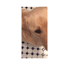
サンプル イメージを読み取って表示します。各種イメージ拡張の効果を比較するために、各変換において同じ入力イメージを使用します。

imOriginal = imresize(imread("kobi.png"),0.25);
imshow(imOriginal)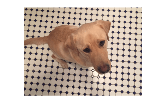 

ランダムなイメージ ワーピング変換

関数 randomAffine2d は、回転、平行移動、スケーリング (サイズ変更)、反転、せん断を組み合わせてランダムな 2 次元アフィン変換を作成します。含める変換、および変換パラメーターの範囲を指定できます。範囲を 2 要素の数値ベクトルとして指定する場合、randomAffine2d は、指定された間隔の一様な確率分布からパラメーターの値を選択します。パラメーター値の範囲をより細かく制御するには、関数ハンドルを使用して範囲を指定できます。

関数 affineOutputView を使用して、imwarp によって作成されたワープ済みイメージの空間範囲と空間分解能を制御します。

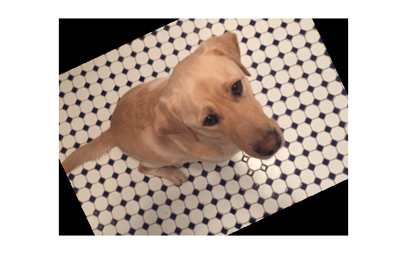
回転

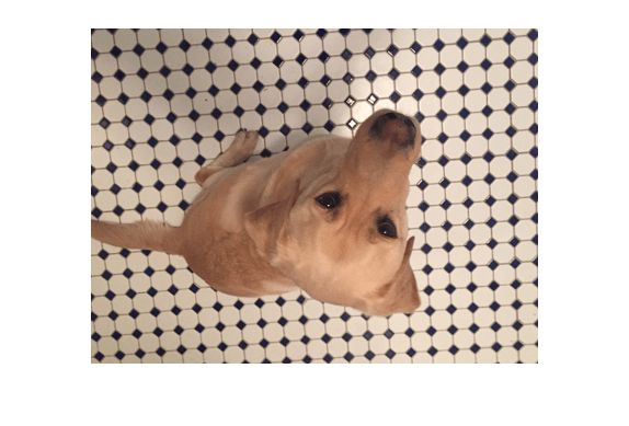
[-45, 45] 度の範囲でランダムに選択した角度によって入力イメージを回転する、ランダムな回転変換を作成します。

tform = randomAffine2d(Rotation=[-45 45]); 
outputView = affineOutputView(size(imOriginal),tform);
imAugmented = imwarp(imOriginal,tform,OutputView=outputView);  
imshow(imAugmented)

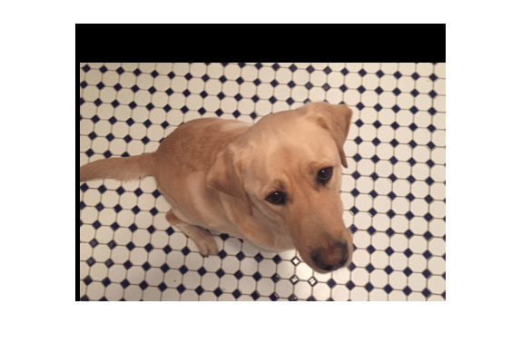
平行移動

[-50, 50] ピクセルの範囲からランダムに選択した距離によって入力イメージを水平および垂直にシフトする、平行移動変換を作成します。

tform = randomAffine2d(XTranslation=[-50 50],YTranslation=[-50 50]);
outputView = affineOutputView(size(imOriginal),tform);
imAugmented = imwarp(imOriginal,tform,OutputView=outputView);
imshow(imAugmented)

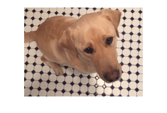
スケール

[1.2, 1.5] の範囲でランダムに選択したスケール係数を使用して入力イメージのサイズを変更する、スケール変換を作成します。この変換は、水平方向と垂直方向に同じ係数を使用してイメージのサイズを変更します。

tform = randomAffine2d(Scale=[1.2,1.5]);
outputView = affineOutputView(size(imOriginal),tform);
imAugmented = imwarp(imOriginal,tform,OutputView=outputView);
imshow(imAugmented)

反転

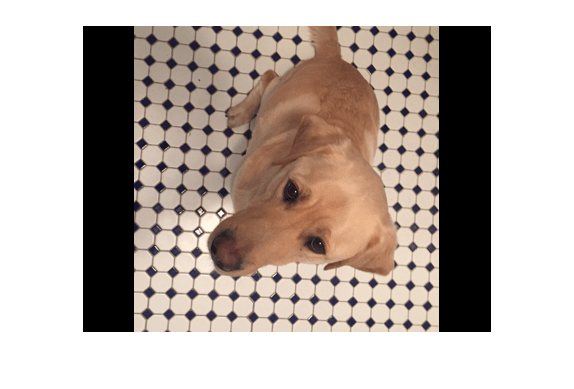
各次元において 50% の確率で入力イメージを反転する、鏡映変換を作成します。

tform = randomAffine2d(XReflection=true,YReflection=true);
outputView = affineOutputView(size(imOriginal),tform);
imAugmented = imwarp(imOriginal,tform,OutputView=outputView);
imshow(imAugmented)

せん断

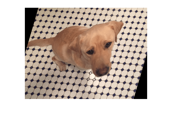
[-30, 30] の範囲からランダムに選択したせん断角度で、水平方向のせん断変換を作成します。

tform = randomAffine2d(XShear=[-30 30]); 
outputView = affineOutputView(size(imOriginal),tform); 
imAugmented = imwarp(imOriginal,tform,OutputView=outputView);
imshow(imAugmented) 

カスタム選択関数を使用した変換パラメーターの範囲の制御

上記の変換では、変換パラメーターの範囲を 2 要素の数値ベクトルによって指定しました。変換パラメーターの範囲をより細かく制御するには、数値ベクトルの代わりに関数ハンドルを指定できます。関数ハンドルは入力引数を取らず、各パラメーターに有効な値を提供します。

たとえば、次のコードは、回転角度 90 度の離散セットから回転角度を選択します。

angles = 0:90:270; 
tform = randomAffine2d(Rotation=@() angles(randi(4))); 
outputView = affineOutputView(size(imOriginal),tform); 
imAugmented = imwarp(imOriginal,tform,OutputView=outputView); 
imshow(imAugmented) 

塗りつぶしの値の制御

幾何学的変換を使用してイメージをワープする場合、出力イメージのピクセルは、入力イメージの境界外の位置にマッピングされることがあります。その場合、imwarp は、出力イメージ内のそれらのピクセルに塗りつぶしの値を割り当てます。既定では、imwarp は塗りつぶしの値に黒を選択します。名前と値の引数 'FillValues' を指定することで、塗りつぶしの値を変更できます。

ランダムな回転変換を作成し、その変換を適用して塗りつぶしの値にグレーを指定します。

tform = randomAffine2d(Rotation=[-45 45]);
outputView = affineOutputView(size(imOriginal),tform);
imAugmented = imwarp(imOriginal,tform,OutputView=outputView, ...
    FillValues=[128 128 128]);
imshow(imAugmented)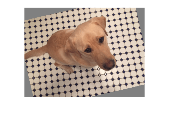

トリミング変換

目的のサイズの出力イメージを作成するには、関数randomWindow2dと関数centerCropWindow2dを使用します。イメージ内の目的の内容が含まれるように注意してウィンドウを選択してください。

トリミングした領域の目的のサイズを、[高さ, 幅] の形式の 2 要素ベクトルとして指定します。

targetSize = [200,100];

イメージの中心から、ターゲット サイズでトリミングします。

win = centerCropWindow2d(size(imOriginal),targetSize); 
imCenterCrop = imcrop(imOriginal,win); 
imshow(imCenterCrop)

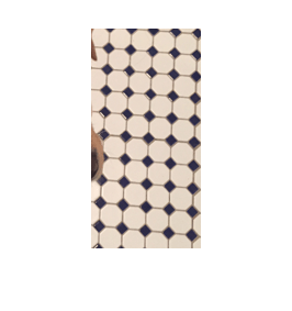
イメージ内のランダムな場所から、ターゲット サイズでイメージをトリミングします。

win = randomWindow2d(size(imOriginal),targetSize);
imRandomCrop = imcrop(imOriginal,win); 
imshow(imRandomCrop)

色変換

関数 jitterColorHSV を使用することにより、カラー イメージの色相、彩度、明度、およびコントラストをランダムに調整できます。含める色変換、および変換パラメーターの範囲を指定できます。

基本的な算術演算を使用することにより、グレースケール イメージの明度とコントラストをランダムに調整できます。

色相ジッター

色相は、色の陰影、またはカラー ホイール上の色の位置を指定します。色相が 0 から 1 まで変化するにつれて、色は赤から黄、緑、シアン、青、紫、マゼンタ、黒と変わり赤に戻ります。色相ジッターは、イメージ内の色に表れる陰影をシフトします。

[0.05, 0.15] の範囲でランダムに選択した小さな正のオフセットにより、入力イメージの色相を調整します。たとえば、赤だった場所がオレンジまたは黄に近づいて見え、オレンジだった場所が黄または緑に見えます。

imJittered = jitterColorHSV(imOriginal,Hue=[0.05 0.15]);
montage({imOriginal,imJittered})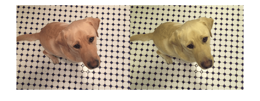

彩度ジッター

彩度は色の純度です。彩度が 0 から 1 まで変化するにつれて、色相はグレー (すべての色の混合を示す) から単一の純色に変化します。彩度ジッターは、色の暗さまたは鮮やかさをシフトします。

[-0.4, -0.1] の範囲でランダムに選択したオフセットにより、入力イメージの彩度を調整します。彩度が下がると、予期したとおり出力イメージの色も弱まります。

imJittered = jitterColorHSV(imOriginal,Saturation=[-0.4 -0.1]); 
montage({imOriginal,imJittered})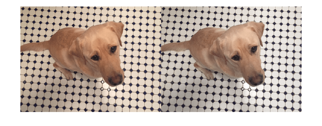

明度ジッター

明度は、色相の量です。明度が 0 から 1 まで変化するにつれて、色は黒から白に変化します。明度ジッターは、入力イメージの暗さと明るさをシフトします。

[-0.3, -0.1] の範囲でランダムに選択したオフセットにより、入力イメージの明度を調整します。明度が下がると、予期したとおりイメージは暗くなります。

imJittered = jitterColorHSV(imOriginal,Brightness=[-0.3 -0.1]); 
montage({imOriginal,imJittered})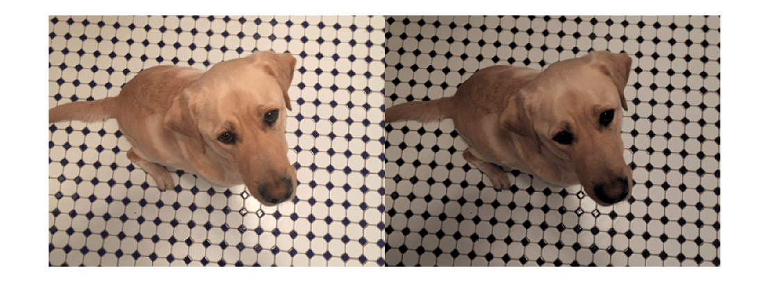

コントラスト ジッター

コントラスト ジッターは、入力イメージの最も暗い領域と最も明るい領域の差異をランダムに調整します。

[1.2, 1.4] の範囲でランダムに選択したスケール係数により、入力イメージのコントラストを調整します。コントラストが強まると、影はより暗くなり、ハイライトはより明るくなります。

imJittered = jitterColorHSV(imOriginal,Contrast=[1.2 1.4]);
montage({imOriginal,imJittered})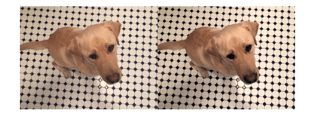

グレースケール イメージの明度およびコントラスト ジッター

基本的な算術演算を使用することにより、ランダムな明度ジッターとコントラスト ジッターをグレースケール イメージに適用できます。

サンプル イメージをグレースケールに変換します。ランダムなコントラスト スケール係数を [0.8, 1] の範囲で指定し、ランダムな明度オフセットを [-0.15, 0.15] の範囲で指定します。イメージをコントラスト スケール係数で乗算してから、明度オフセットを加算します。

imGray = im2gray(im2double(imOriginal)); 
contrastFactor = 1-0.2*rand; 
brightnessOffset = 0.3*(rand-0.5); 
imJittered = imGray.*contrastFactor + brightnessOffset;
imJittered = im2uint8(imJittered);
montage({imGray,imJittered})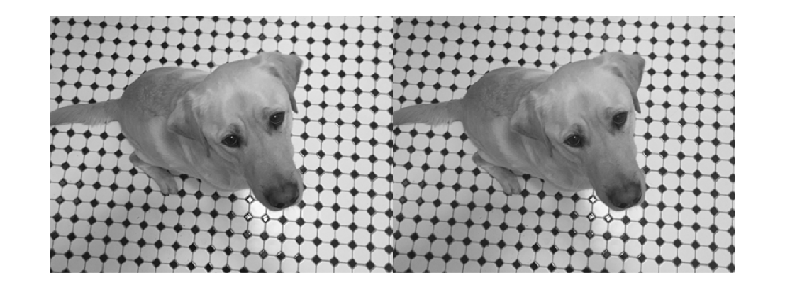

カラーからグレースケールへのランダム変換

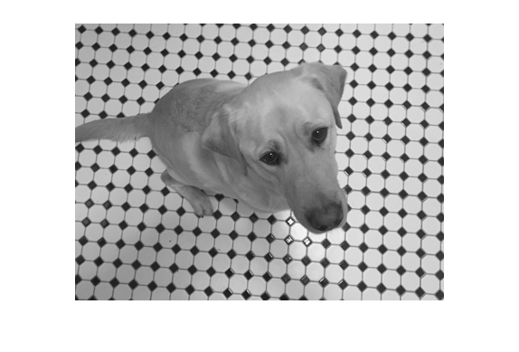
色拡張の 1 タイプでは、ネットワークに必要なチャネル数を保持しながら、RGB イメージから色情報をランダムに破棄します。次のコードは "ランダム グレースケール" 変換を示します。ここでは RGB イメージが 80% の確率で 3 チャネルの出力イメージ (R == G == B) にランダムに変換されます。

desiredProbability = 0.8;
if rand <= desiredProbability
    imJittered = repmat(rgb2gray(imOriginal),[1 1 3]);
end
imshow(imJittered) 

その他のイメージ処理演算

関数 transform を使用して、Image Processing Toolbox 関数の任意の組み合わせを入力イメージに適用します。ノイズとぼかしの追加は、深層学習アプリケーションで使用される一般的なイメージ処理演算のうちの 2 つです。

合成ノイズ

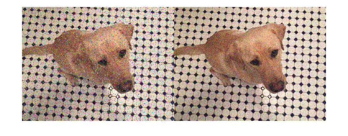
合成ノイズを入力イメージに適用するには、関数 imnoise を使用します。ガウス ノイズ、ポアソン ノイズ、ごま塩ノイズ、乗法性ノイズなど、使用するノイズ モデルを指定できます。ノイズの強度を指定することもできます。

imSaltAndPepperNoise = imnoise(imOriginal,"salt & pepper",0.1);
imGaussianNoise = imnoise(imOriginal,"gaussian");
montage({imSaltAndPepperNoise,imGaussianNoise}) 

合成ぼかし

ランダムなガウスぼかしをイメージに適用するには、関数 imgaussfilt を使用します。平滑化の量を指定できます。

sigma = 1+5*rand; 
imBlurred = imgaussfilt(imOriginal,sigma); 
imshow(imBlurred)

データストア内のイメージ データへの拡張の適用

実用的な深層学習の問題においては、通常、イメージ拡張パイプラインでは複数の演算を組み合わせます。データストアは、イメージ コレクションの読み取りや拡張に便利です。

例のこのセクションでは、イメージ分類およびイメージ回帰の問題のための学習のコンテキストでデータストアを拡張する、データ拡張パイプラインの定義方法を示します。

まず、未処理のイメージを含む imageDatastore を作成します。この例のイメージ データストアには、ラベル付きの数字のイメージが含まれています。

digitDatasetPath = fullfile(matlabroot,"toolbox","nnet", ...
    "nndemos","nndatasets","DigitDataset");
imds = imageDatastore(digitDatasetPath, ...
    IncludeSubfolders=true,LabelSource="foldernames");
imds.ReadSize = 6;

イメージ分類

イメージ分類では、イメージにランダムな変更が加えられていても、これが依然として同じイメージ クラスを表していることを分類器が学習しなければなりません。イメージ分類のためにデータを拡張するには、対応するカテゴリカル ラベルに変更を加えずに入力イメージを拡張するだけで十分です。

ランダムなガウスぼかし、ごま塩ノイズ、およびランダムなスケーリングと回転を使用して、初期状態のイメージ データストア内のイメージを拡張します。これらの演算は、この例の終わりにある補助関数 classificationAugmentationPipeline で定義されます。関数 transform を使用して、学習データにデータ拡張を適用します。

dsTrain = transform(imds,@classificationAugmentationPipeline, ...
    IncludeInfo=true);

拡張されたパイプラインからの出力のサンプルを可視化します。

dataPreview = preview(dsTrain);
montage(dataPreview(:,1))
title("Augmented Images for Image Classification")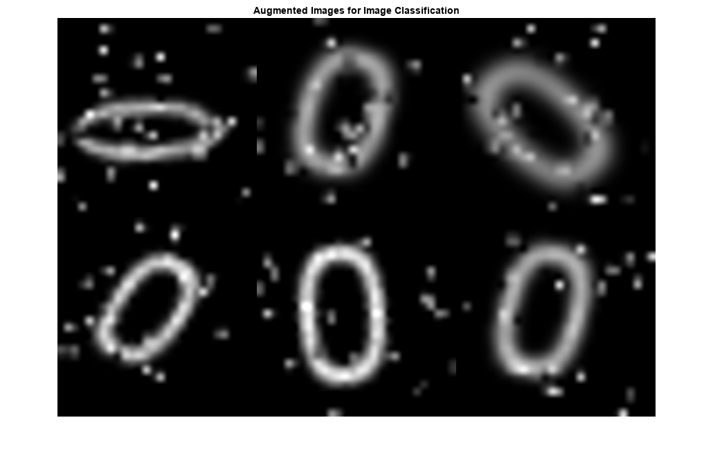

イメージ回帰

image-to-image 回帰のイメージ拡張は入力イメージと応答イメージに対して同一の幾何学的変換を適用しなければならないため、さらに複雑です。関数 combine を使用して、入力イメージと応答イメージのペアを関連付けます。関数 transform を使用して、各ペアの一方または両方のイメージを変換します。

イメージ データストア imds の同一な 2 つのコピーを結合します。結合したデータストアからデータを読み取ると、イメージ データが 2 列の cell 配列で返されます。ここで最初の列はネットワークの入力イメージを表し、2 番目の列にはネットワークの応答が格納されます。

dsCombined = combine(imds,imds);
montage(preview(dsCombined)',Size=[6 2])
title("Combined Input and Response Pairs Before Augmentation")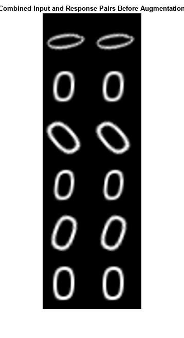

一連のイメージ処理演算を使用して、学習イメージの各ペアを拡張します。

• 入力イメージと応答イメージのサイズを 32 x 32 ピクセルに変更。

• 入力イメージにのみごま塩ノイズを付加。

• スケールと回転をランダムに行う変換を作成。

• 入力イメージと応答イメージに同じ変換を適用。

これらの演算は、この例の終わりにある補助関数 imageRegressionAugmentationPipeline で定義されます。関数 transform を使用して、学習データにデータ拡張を適用します。

dsTrain = transform(dsCombined,@imageRegressionAugmentationPipeline);
montage(preview(dsTrain)',Size=[6 2])
title("Combined Input and Response Pairs After Augmentation")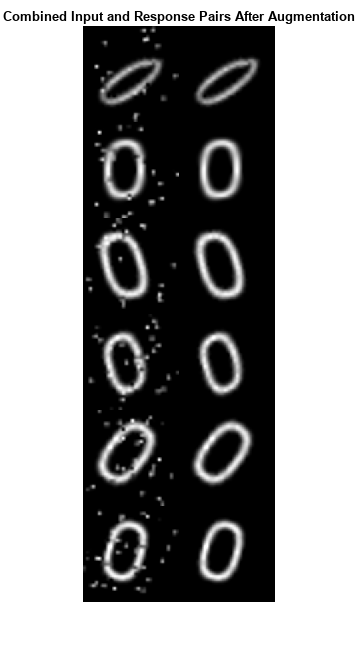

image-to-image 回帰ネットワークの学習と評価に関する詳細な例については、image-to-image 回帰用のデータストアの準備 (Deep Learning Toolbox)を参照してください。

サポート関数

補助関数 classificationAugmentationPipeline は、分類用にイメージを拡張します。dataIn と dataOut は 2 要素の cell 配列で、最初の要素がネットワークの入力イメージ、2 番目の要素がカテゴリカル ラベルです。

function [dataOut,info] = classificationAugmentationPipeline(dataIn,info)

dataOut = cell([size(dataIn,1),2]);

for idx = 1:size(dataIn,1)
    temp = dataIn{idx};
    
    % Add randomized Gaussian blur
    temp = imgaussfilt(temp,1.5*rand);
    
    % Add salt and pepper noise
    temp = imnoise(temp,"salt & pepper");
    
    % Add randomized rotation and scale
    tform = randomAffine2d(Scale=[0.95,1.05],Rotation=[-30 30]);
    outputView = affineOutputView(size(temp),tform);
    temp = imwarp(temp,tform,OutputView=outputView);
    
    % Form a two-element cell array with the input image and expected response
    dataOut(idx,:) = {temp,info.Label(idx)};
end

end

補助関数 imageRegressionAugmentationPipeline は、image-to-image 回帰用にイメージを拡張します。dataIn と dataOut は 2 要素の cell 配列です。配列の最初の要素はネットワークの入力イメージで、2 番目の要素はネットワークの応答イメージです。

function dataOut = imageRegressionAugmentationPipeline(dataIn)

dataOut = cell([size(dataIn,1),2]);
for idx = 1:size(dataIn,1)
    
    % Resize images to 32-by-32 pixels and convert to data type single
    inputImage = im2single(imresize(dataIn{idx,1},[32 32]));
    targetImage = im2single(imresize(dataIn{idx,2},[32 32]));
    
    % Add salt and pepper noise
    inputImage = imnoise(inputImage,"salt & pepper");
    
    % Add randomized rotation and scale
    tform = randomAffine2d(Scale=[0.9,1.1],Rotation=[-30 30]);
    outputView = affineOutputView(size(inputImage),tform);
    
    % Use imwarp with the same tform and outputView to augment both images
    % the same way
    inputImage = imwarp(inputImage,tform,OutputView=outputView);
    targetImage = imwarp(targetImage,tform,OutputView=outputView);
    
    dataOut(idx,:) = {inputImage,targetImage};
end

end

参考

transform | combine

関連する例

• image-to-image 回帰用のデータストアの準備 (Deep Learning Toolbox)

詳細

• 深層学習用イメージ前処理とイメージ拡張の入門
• イメージの深層学習向け前処理