showStateInfo
スパース モデルの状態ベクトルのマッピング
説明
showStateInfo( は、ベクトル sys)x または q の状態ベクトルのマッピング、つまりそれらがコンポーネント、インターフェイス、および信号にどのように分割されるかを出力します。
sparss モデルの場合、showStateInfo は、状態ベクトル x の内容を個々のコンポーネントおよび内部信号にマッピングします。ここで、Component は sys に結合されたサブコンポーネントまたはサブ構造を示します。Signal グループには、直列接続やフィードバック接続など、コンポーネント間を流れるすべての信号が含まれます。
mechss モデルの場合、showStateInfo は、一般化された自由度のベクトル q の内容をコンポーネント、インターフェイス、および信号のそれぞれについてマッピングします。Interface グループには、コンポーネント間の物理結合から生じるすべての DAE 変数が含まれます (addInterface および assemble を参照)。
例
この例では、スパース 2 次モデルを含む sparseSOSignal.mat について考えます。アクチュエータ、センサー、コントローラーを定義して、それらをフィードバック ループでプラントに接続します。
スパース行列を読み込み、mechss オブジェクトを作成します。
load sparseSOSignal.mat
plant = mechss(M,C,K,B,F,[],[],'Name','Plant');
次に、伝達関数を使用してアクチュエータとセンサーを作成します。
act = tf(1,[1 0.5 3],'Name','Actuator');
sen = tf(1,[0.02 7],'Name','Sensor');
プラントの PID コントローラー オブジェクトを作成します。
con = pid(1,1,0.1,0.01,'Name','Controller');
feedback コマンドを使用して、プラント、センサー、アクチュエータ、およびコントローラーをフィードバック ループ内で接続します。
sys = feedback(sen*plant*act*con,1)
Sparse continuous-time second-order model with 1 outputs, 1 inputs, and 7111 degrees of freedom.
Model Properties

Use "spy" and "showStateInfo" to inspect model structure.
Type "help mechssOptions" for available solver options for this model.
mechss オブジェクトがどのモデル オブジェクト タイプよりも優先されるため、結果のシステム sys は mechss オブジェクトになります。
showStateInfo を使用してコンポーネントと信号グループを表示します。
showStateInfo(sys)
The state groups are:

    Type          Name       Size
  -------------------------------
  Component      Sensor         1
  Component      Plant       7102
  Signal                        1
  Component     Actuator        2
  Signal                        1
  Component    Controller       2
  Signal                        1
  Signal                        1
xsort を使用してコンポーネントと信号を並べ替えてから、コンポーネントと信号グループを表示します。
sysSort = xsort(sys);
showStateInfo(sysSort)
The state groups are:

    Type          Name       Size
  -------------------------------
  Component      Sensor         1
  Component      Plant       7102
  Component     Actuator        2
  Component    Controller       2
  Signal                        4
コンポーネントが信号区分の前に順序付けされていることを確認します。信号は並べ替えられて、単一の区分にグループ化されます。
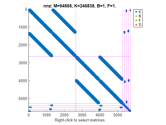
spy を使用して結果のシステムのスパース パターンを可視化することもできます。
spy(sysSort)

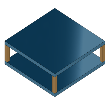
この例では、下の図に示すように、各頂点の支柱に連結されている 2 枚の四角形のプレートで構成される構造モデルを考えます。下のプレートは地面にしっかり取り付けられ、支柱は四角形のプレートの各頂点にしっかり取り付けられています。
platePillarModel.mat に含まれている有限要素モデル行列を読み込み、上記システムを表すスパース 2 次モデルを作成します。
load('platePillarModel.mat')インターフェイスを定義します。
Plate1 = mechss(M1,[],K1,B1,F1,'Name','Plate1');
Plate2 = mechss(M2,[],K2,B2,F2,'Name','Plate2');
次に、相互作用する自由度 (DOF) インデックス データを dofData.mat から読み込み、interface を使用して 2 枚のプレートと 4 本の支柱間の物理的接続を作成します。dofs は、最初の 2 行に 1 枚目と 2 枚目のプレートの DOF インデックス データを含み、他の 4 行に 4 本の支柱のインデックス データを含む 6x7 の cell 配列です。関数は既定で、物理結合のデュアルアセンブリ メソッドを使用します。
load('dofData.mat','dofs')
for ct=1:4
    % Plates to pillars
    Plate1 = addInterface(Plate1,"Pillar"+ct,dofs{1,2+ct});
    Plate2 = addInterface(Plate2,"Pillar"+ct,dofs{2,2+ct});
end

P = cell(4,1);
for ct=1:4
    % Pillars to plates
    P{ct} = mechss(Mp,[],Kp,Bp,Fp,'Name',"Pillar"+ct);
    P{ct} = addInterface(P{ct},"TopMount",dofs{2+ct,1});
    P{ct} = addInterface(P{ct},"BottomMount",dofs{2+ct,2});
end
% Plate 2 to ground
下のプレートと地面間の接続を指定します。
Plate2 = addInterface(Plate2,"Ground",dofs{2,7});

% Assemble
model = append(Plate1,Plate2,P{:});
物理インターフェイスを確認するには showStateInfo を使用します。
showStateInfo(model)
The state groups are:

    Type        Name      Size
  ----------------------------
  Component    Plate1     2646
  Component    Plate2     2646
  Component    Pillar1     132
  Component    Pillar2     132
  Component    Pillar3     132
  Component    Pillar4     132
sysConDual = model;
for ct=1:4
    sysConDual = assemble(sysConDual,"Plate1:Pillar"+ct,"Pillar"+ct+":TopMount"');
    sysConDual = assemble(sysConDual,"Plate2:Pillar"+ct,"Pillar"+ct+":BottomMount");
end
sysConDual = assemble(sysConDual,"Plate2:Ground","Ground");
物理インターフェイスを確認するには showStateInfo を使用します。
showStateInfo(sysConDual)
The state groups are:

    Type                      Name                   Size
  -------------------------------------------------------
  Component                  Plate1                  2646
  Component                  Plate2                  2646
  Component                 Pillar1                   132
  Component                 Pillar2                   132
  Component                 Pillar3                   132
  Component                 Pillar4                   132
  Interface     Plate1:Pillar1-Pillar1:TopMount        12
  Interface    Plate2:Pillar1-Pillar1:BottomMount      12
  Interface     Plate1:Pillar2-Pillar2:TopMount        12
  Interface    Plate2:Pillar2-Pillar2:BottomMount      12
  Interface     Plate1:Pillar3-Pillar3:TopMount        12
  Interface    Plate2:Pillar3-Pillar3:BottomMount      12
  Interface     Plate1:Pillar4-Pillar4:TopMount        12
  Interface    Plate2:Pillar4-Pillar4:BottomMount      12
  Interface           Plate2:Ground-Ground              6
spy を使用して、最終モデルのスパース行列を可視化できます。
spy(sysConDual)

ここで、主要アセンブリ メソッドを使用して物理的接続を指定します。
sysConPrimal = model;
for ct=1:4
    sysConPrimal = assemble(sysConPrimal,"Plate1:Pillar"+ct,"Pillar"+ct+":TopMount"',Method="primal");
    sysConPrimal = assemble(sysConPrimal,"Plate2:Pillar"+ct,"Pillar"+ct+":BottomMount",Method="primal");
end
sysConPrimal = assemble(sysConPrimal,"Plate2:Ground","Ground",Method="primal");
物理インターフェイスを確認するには showStateInfo を使用します。
showStateInfo(sysConPrimal)
The state groups are:

    Type       Name    Size
  -------------------------
  Component            5718
主要アセンブリによって、グローバル有限要素メッシュ内の一連の共有 DOF に関連付けられた冗長な DOF の半分が取り除かれます。
spy を使用して、最終モデルのスパース行列を可視化できます。
spy(sysConPrimal)
この例のデータセットは、ASML の Victor Dolk によって提供されています。
入力引数
バージョン履歴
R2020b で導入