結果:
t = turtle(); % Start a turtle
t.forward(100); % Move forward by 100
t.backward(100); % Move backward by 100
t.left(90); % Turn left by 90 degrees
t.right(90); % Tur right by 90 degrees
t.goto(100, 100); % Move to (100, 100)
t.turnto(90); % Turn to 90 degrees, i.e. north
t.speed(1000); % Set turtle speed as 1000 (default: 500)
t.pen_up(); % Pen up. Turtle leaves no trace.
t.pen_down(); % Pen down. Turtle leaves a trace again.
t.color('b'); % Change line color to 'b'
t.begin_fill(FaceColor, EdgeColor, FaceAlpha); % Start filling
t.end_fill(); % End filling
t.change_icon('person.png'); % Change the icon to 'person.png'
t.clear(); % Clear the Axes
classdef turtle < handle
properties (GetAccess = public, SetAccess = private)
x = 0
y = 0
q = 0
end
properties (SetAccess = public)
speed (1, 1) double = 500
end
properties (GetAccess = private)
speed_reg = 100
n_steps = 20
ax
l
ht
im
is_pen_up = false
is_filling = false
fill_color
fill_alpha
end
methods
function obj = turtle()
figure(Name='MATurtle', NumberTitle='off')
obj.ax = axes(box="on");
hold on,
obj.ht = hgtransform();
icon = flipud(imread('turtle.png'));
obj.im = imagesc(obj.ht, icon, ...
XData=[-30, 30], YData=[-30, 30], ...
AlphaData=(255 - double(rgb2gray(icon)))/255);
obj.l = plot(obj.x, obj.y, 'k');
obj.ax.XLim = [-500, 500];
obj.ax.YLim = [-500, 500];
obj.ax.DataAspectRatio = [1, 1, 1];
obj.ax.Toolbar.Visible = 'off';
disableDefaultInteractivity(obj.ax);
end
function home(obj)
obj.x = 0;
obj.y = 0;
obj.ht.Matrix = eye(4);
end
function forward(obj, dist)
obj.step(dist);
end
function backward(obj, dist)
obj.step(-dist)
end
function step(obj, delta)
if numel(delta) == 1
delta = delta*[cosd(obj.q), sind(obj.q)];
end
if obj.is_filling
obj.fill(delta);
else
obj.move(delta);
end
end
function goto(obj, x, y)
dx = x - obj.x;
dy = y - obj.y;
obj.turnto(rad2deg(atan2(dy, dx)));
obj.step([dx, dy]);
end
function left(obj, q)
obj.turn(q);
end
function right(obj, q)
obj.turn(-q);
end
function turnto(obj, q)
obj.turn(obj.wrap_angle(q - obj.q, -180));
end
function pen_up(obj)
if obj.is_filling
warning('not available while filling')
return
end
obj.is_pen_up = true;
end
function pen_down(obj, go)
if obj.is_pen_up
if nargin == 1
obj.l(end+1) = plot(obj.x, obj.y, Color=obj.l(end).Color);
else
obj.l(end+1) = go;
end
uistack(obj.ht, 'top')
end
obj.is_pen_up = false;
end
function color(obj, line_color)
if obj.is_filling
warning('not available while filling')
return
end
obj.pen_up();
obj.pen_down(plot(obj.x, obj.y, Color=line_color));
end
function begin_fill(obj, FaceColor, EdgeColor, FaceAlpha)
arguments
obj
FaceColor = [.6, .9, .6];
EdgeColor = [0 0.4470 0.7410];
FaceAlpha = 1;
end
if obj.is_filling
warning('already filling')
return
end
obj.fill_color = FaceColor;
obj.fill_alpha = FaceAlpha;
obj.pen_up();
obj.pen_down(patch(obj.x, obj.y, [1, 1, 1], ...
EdgeColor=EdgeColor, FaceAlpha=0));
obj.is_filling = true;
end
function end_fill(obj)
if ~obj.is_filling
warning('not filling now')
return
end
obj.l(end).FaceColor = obj.fill_color;
obj.l(end).FaceAlpha = obj.fill_alpha;
obj.is_filling = false;
end
function change_icon(obj, filename)
icon = flipud(imread(filename));
obj.im.CData = icon;
obj.im.AlphaData = (255 - double(rgb2gray(icon)))/255;
end
function clear(obj)
obj.x = 0;
obj.y = 0;
delete(obj.ax.Children(2:end));
obj.l = plot(0, 0, 'k');
obj.ht.Matrix = eye(4);
end
end
methods (Access = private)
function animated_step(obj, delta, q, initFcn, updateFcn)
arguments
obj
delta
q
initFcn = @() []
updateFcn = @(~, ~) []
end
dx = delta(1)/obj.n_steps;
dy = delta(2)/obj.n_steps;
dq = q/obj.n_steps;
pause_duration = norm(delta)/obj.speed/obj.speed_reg;
initFcn();
for i = 1:obj.n_steps
updateFcn(dx, dy);
obj.ht.Matrix = makehgtform(...
translate=[obj.x + dx*i, obj.y + dy*i, 0], ...
zrotate=deg2rad(obj.q + dq*i));
pause(pause_duration)
drawnow limitrate
end
obj.x = obj.x + delta(1);
obj.y = obj.y + delta(2);
end
function obj = turn(obj, q)
obj.animated_step([0, 0], q);
obj.q = obj.wrap_angle(obj.q + q, 0);
end
function move(obj, delta)
initFcn = @() [];
updateFcn = @(dx, dy) [];
if ~obj.is_pen_up
initFcn = @() initializeLine();
updateFcn = @(dx, dy) obj.update_end_point(obj.l(end), dx, dy);
end
function initializeLine()
obj.l(end).XData(end+1) = obj.l(end).XData(end);
obj.l(end).YData(end+1) = obj.l(end).YData(end);
end
obj.animated_step(delta, 0, initFcn, updateFcn);
end
function obj = fill(obj, delta)
initFcn = @() initializePatch();
updateFcn = @(dx, dy) obj.update_end_point(obj.l(end), dx, dy);
function initializePatch()
obj.l(end).Vertices(end+1, :) = obj.l(end).Vertices(end, :);
obj.l(end).Faces = 1:size(obj.l(end).Vertices, 1);
end
obj.animated_step(delta, 0, initFcn, updateFcn);
end
end
methods (Static, Access = private)
function update_end_point(l, dx, dy)
l.XData(end) = l.XData(end) + dx;
l.YData(end) = l.YData(end) + dy;
end
function q = wrap_angle(q, min_angle)
q = mod(q - min_angle, 360) + min_angle;
end
end
end
I would like to zoom directly on the selected region when using  on my image created with image or imagesc. First of all, I would recommend using image or imagesc and not imshow for this case, see comparison here: Differences between imshow() and image()? However when zooming Stretch-to-Fill behavior happens and I don't want that. Try range zoom to image generated by this code:
fig = uifigure;
ax = uiaxes(fig);
im = imread("peppers.png");
h = imagesc(im,"Parent",ax);
axis(ax,'tight', 'off')
I can fix that with manualy setting data aspect ratio:
daspect(ax,[1 1 1])
However, I need this code to run automatically after zooming. So I create zoom object and ActionPostCallback which is called everytime after I zoom, see zoom - ActionPostCallback.
z = zoom(ax);
z.ActionPostCallback = @(fig,ax) daspect(ax.Axes,[1 1 1]);
If you need, you can also create ActionPreCallback which is called everytime before I zoom, see zoom - ActionPreCallback.
z.ActionPreCallback = @(fig,ax) daspect(ax.Axes,'auto');
Code written and run in R2025a.
I am thrilled python interoperability now seems to work for me with my APPLE M1 MacBookPro and MATLAB V2025a. The available instructions are still, shall we say, cryptic. Here is a summary of my interaction with GPT 4o to get this to work.
===========================================================
MATLAB R2025a + Python (Astropy) Integration on Apple Silicon (M1/M2/M3 Macs)
===========================================================
Author: D. Carlsmith, documented with ChatGPT
Last updated: July 2025
This guide provides full instructions, gotchas, and workarounds to run Python 3.10 with MATLAB R2025a (Apple Silicon/macOS) using native ARM64 Python and calling modules like Astropy, Numpy, etc. from within MATLAB.
===========================================================
Overview
===========================================================
- MATLAB R2025a on Apple Silicon (M1/M2/M3) runs as "maca64" (native ARM64).
- To call Python from MATLAB, the Python interpreter must match that architecture (ARM64).
- Using Intel Python (x86_64) with native MATLAB WILL NOT WORK.
- The cleanest solution: use Miniforge3 (Conda-forge's lightweight ARM64 distribution).
===========================================================
1. Install Miniforge3 (ARM64-native Conda)
===========================================================
In Terminal, run:
curl -LO https://github.com/conda-forge/miniforge/releases/latest/download/Miniforge3-MacOSX-arm64.sh
bash Miniforge3-MacOSX-arm64.sh
Follow prompts:
- Press ENTER to scroll through license.
- Type "yes" when asked to accept the license.
- Press ENTER to accept the default install location: ~/miniforge3
- When asked:
Do you wish to update your shell profile to automatically initialize conda? [yes|no]
Type: yes
===========================================================
2. Restart Terminal and Create a Python Environment for MATLAB
===========================================================
Run the following:
conda create -n matlab python=3.10 astropy numpy -y
conda activate matlab
Verify the Python path:
which python
Expected output:
/Users/YOURNAME/miniforge3/envs/matlab/bin/python
===========================================================
3. Verify Python + Astropy From Terminal
===========================================================
Run:
python -c "import astropy; print(astropy.__version__)"
Expected output:
6.x.x (or similar)
===========================================================
4. Configure MATLAB to Use This Python
===========================================================
In MATLAB R2025a (Apple Silicon):
clear classes
pyenv('Version', '/Users/YOURNAME/miniforge3/envs/matlab/bin/python')
py.sys.version
You should see the Python version printed (e.g. 3.10.18). No error means it's working.
===========================================================
5. Gotchas and Their Solutions
===========================================================
❌ Error: Python API functions are not available
→ Cause: Wrong architecture or broken .dylib
→ Fix: Use Miniforge ARM64 Python. DO NOT use Intel Anaconda.
❌ Error: Invalid text character (↑ points at __version__)
→ Cause: MATLAB can’t parse double underscores typed or pasted
→ Fix: Use: py.getattr(module, '__version__')
❌ Error: Unrecognized method 'separation' or 'sec'
→ Cause: MATLAB can't reflect dynamic Python methods
→ Fix: Use: py.getattr(obj, 'method')(args)
===========================================================
6. Run Full Verification in MATLAB
===========================================================
Paste this into MATLAB:
% Set environment
clear classes
pyenv('Version', '/Users/YOURNAME/miniforge3/envs/matlab/bin/python');
% Import modules
coords = py.importlib.import_module('astropy.coordinates');
time_mod = py.importlib.import_module('astropy.time');
table_mod = py.importlib.import_module('astropy.table');
% Astropy version
ver = char(py.getattr(py.importlib.import_module('astropy'), '__version__'));
disp(['Astropy version: ', ver]);
% SkyCoord angular separation
c1 = coords.SkyCoord('10h21m00s', '+41d12m00s', pyargs('frame', 'icrs'));
c2 = coords.SkyCoord('10h22m00s', '+41d15m00s', pyargs('frame', 'icrs'));
sep_fn = py.getattr(c1, 'separation');
sep = sep_fn(c2);
arcsec = double(sep.to('arcsec').value);
fprintf('Angular separation = %.3f arcsec\n', arcsec);
% Time difference in seconds
Time = time_mod.Time;
t1 = Time('2025-01-01T00:00:00', pyargs('format','isot','scale','utc'));
t2 = Time('2025-01-02T00:00:00', pyargs('format','isot','scale','utc'));
dt = py.getattr(t2, '__sub__')(t1);
seconds = double(py.getattr(dt, 'sec'));
fprintf('Time difference = %.0f seconds\n', seconds);
% Astropy table display
tbl = table_mod.Table(pyargs('names', {'a','b'}, 'dtype', {'int','float'}));
tbl.add_row({1, 2.5});
tbl.add_row({2, 3.7});
disp(tbl);
===========================================================
7. Optional: Automatically Configure Python in startup.m
===========================================================
To avoid calling pyenv() every time, edit your MATLAB startup:
edit startup.m
Add:
try
pyenv('Version', '/Users/YOURNAME/miniforge3/envs/matlab/bin/python');
catch
warning("Python already loaded.");
end
===========================================================
8. Final Notes
===========================================================
- This setup avoids all architecture mismatches.
- It uses a clean, minimal ARM64 Python that integrates seamlessly with MATLAB.
- Do not mix Anaconda (Intel) with Apple Silicon MATLAB.
- Use py.getattr for any Python attribute containing underscores or that MATLAB can't resolve.
You can now run NumPy, Astropy, Pandas, Astroquery, Matplotlib, and more directly from MATLAB.
===========================================================
群馬産業技術センター様をお招きし、製造現場での異常検知の取り組みについてご紹介いただくオンラインセミナーを開催します。
実際の開発事例を通して、MATLABを使った「教師なし」異常検知の進め方や、予知保全に役立つ最新機能もご紹介します。
✅ 異常検知・予知保全に興味がある方
✅ データ活用を何から始めればいいか迷っている方
✅ 実際の現場事例を知りたい方
ぜひお気軽にご参加ください!
Hey MATLAB enthusiasts!
I just stumbled upon this hilariously effective GitHub repo for image deformation using Moving Least Squares (MLS)—and it’s pure gold for anyone who loves playing with pixels! 🎨✨
- Real-Time Magic ✨
- Precomputes weights and deformation data upfront, making it blazing fast for interactive edits. Drag control points and watch the image warp like rubber! (2)
- Supports affine, similarity, and rigid deformations—because why settle for one flavor of chaos?
- Single-File Simplicity 🧩
- All packed into one clean MATLAB class (mlsImageWarp.m).
- Endless Fun Use Cases 🤹
- Turn your pet’s photo into a Picasso painting.
- "Fix" your friend’s smile... aggressively.
- Animate static images with silly deformations (1).
Try the Demo!
You are not a jedi yet !
20%
We not grant u the rank of master !
0%
Ready are u? What knows u of ready?
0%
May the Force be with you !
80%
5 票
Simulinkモデルを生成AIで自動的に作成できたら便利だと思いませんか?
QiitaのSacredTubesさんは、このアイデアを実験的に試みた記事を公開しています。
その方法は、まず生成AIでVerilogコードを作成し、それをSimulinkに取り込んでモデル化するというものです。(ここではHDL Coderというツールボックスの機能が使われました:importhdl)
まだ実用段階には至っていませんが、モデルベース開発(MBD)と生成AIの可能性を探る上で、非常に興味深い試みです。
生成AIの限界と可能性を考えるきっかけとして、一読の価値があります。
---
もし「Simulink Copilot」のような生成AIツールが登場するとしたら、
どんな機能があったら嬉しいと思いますか?
- 自然言語でブロック図を生成?
- 既存モデルの自動ドキュメント化?
- シミュレーション結果の要約と解釈?
皆さんのアイデアをぜひシェアしてください!
- 昨日までちゃんと動いていたのに・・
- ヘルプページ通りに書いているのに・・
MATLAB 関数がエラーを出すようになることありますよね(?)そんな時にみなさんがまず確認するもの、何かありますか?教えてください!
例えば
which -all plot
をコマンドウィンドウで実行して、もともと MATLAB で定義されている plot 関数(MATLAB のインストールフォルダにある plot 関数)がちゃんと頭に出てくるかどうか確認します。
キーと値の組み合わせでデータを格納できるディクショナリ。R2022bでdictionaryコマンドが登場し、最近のバージョンではreaddictionaryとwritedictionaryでJSONファイルからの読み込み・書き込みにも対応しました。
私はMIDIデータからピアノの演奏動画を作るプログラムで、ディクショナリを使いました。音のノート番号をキーにして、patchで白と黒で鍵盤を塗りつぶしたmatlab.graphics.Graphicsデータ型を値にしたディクショナリで保存して、MIDIで鳴らされた音のノート番号からlookupでグラフのオブジェクトを取得し、FaceColorを変更してハイライトするというもの。
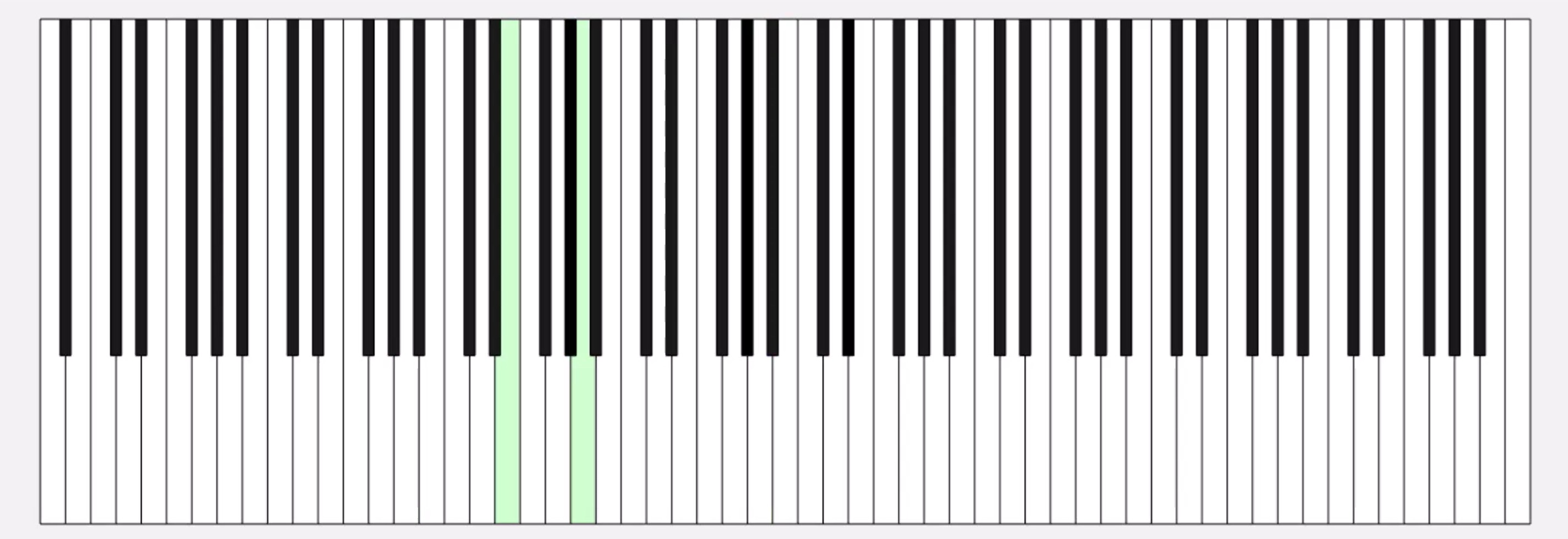
コード例
%% MIDIデータの.matファイルを読み取ってピアノを描画するサンプル
fig = figure('Position', [34 328 1626 524]);
ax = axes;
whiteKeyY = [0 0 150 150];
whiteKeyColor = [1 1 1];
blackKeyY = [50 50 150 150];
blackKeyColor = [0.1 0.1 0.1];
edgeColor = [0 0 0];
% ディクショナリの定義
d = configureDictionary("double", "matlab.graphics.Graphics");
% 白鍵を描画
for n = 1:9
pos = 23*7*(n-1);
d = insert(d, 21 + (n-1)*12, patch([pos+5 pos+28 pos+28 pos+5],whiteKeyY, whiteKeyColor, 'EdgeColor', edgeColor, 'UserData', 21 + (n-1)*12));
d = insert(d, 23 + (n-1)*12, patch([pos+28 pos+51 pos+51 pos+28], whiteKeyY, whiteKeyColor, 'EdgeColor', edgeColor, 'UserData', 23 + (n-1)*12));
d = insert(d, 24 + (n-1)*12, patch([pos+51 pos+74 pos+74 pos+51], whiteKeyY, whiteKeyColor, 'EdgeColor', edgeColor, 'UserData', 24 + (n-1)*12));
if n < 9
d = insert(d, 26 + (n-1)*12, patch([pos+74 pos+97 pos+97 pos+74], whiteKeyY, whiteKeyColor, 'EdgeColor', edgeColor, 'UserData', 26 + (n-1)*12));
d = insert(d, 28 + (n-1)*12, patch([pos+97 pos+120 pos+120 pos+97], whiteKeyY, whiteKeyColor, 'EdgeColor', edgeColor, 'UserData', 28 + (n-1)*12));
d = insert(d, 29 + (n-1)*12, patch([pos+120 pos+143 pos+143 pos+120], whiteKeyY, whiteKeyColor, 'EdgeColor', edgeColor, 'UserData', 29 + (n-1)*12));
d = insert(d, 31 + (n-1)*12, patch([pos+143 pos+166 pos+166 pos+143], whiteKeyY, whiteKeyColor, 'EdgeColor', edgeColor, 'UserData', 31 + (n-1)*12));
end
end
% 黒鍵を描画。白鍵の上になるようにループを分けています
for n = 1:9
pos = 23*7*(n-1);
d = insert(d, 22 + (n-1)*12, patch([pos+23 pos+33 pos+33 pos+23], blackKeyY, blackKeyColor, 'EdgeColor', [0 0 0], 'UserData', 22 + (n-1)*12));
if n < 9
d = insert(d, 25 + (n-1)*12, patch([pos+69 pos+79 pos+79 pos+69], blackKeyY, blackKeyColor, 'EdgeColor', [0 0 0], 'UserData', 25 + (n-1)*12));
d = insert(d, 27 + (n-1)*12, patch([pos+92 pos+102 pos+102 pos+92], blackKeyY, blackKeyColor, 'EdgeColor', [0 0 0], 'UserData', 27 + (n-1)*12));
d = insert(d, 30 + (n-1)*12, patch([pos+138 pos+148 pos+148 pos+138], blackKeyY, blackKeyColor, 'EdgeColor', [0 0 0], 'UserData', 30 + (n-1)*12));
d = insert(d, 32 + (n-1)*12, patch([pos+161 pos+171 pos+171 pos+161], blackKeyY, blackKeyColor, 'EdgeColor', [0 0 0], 'UserData', 32 + (n-1)*12));
end
end
xticklabels({})
yticklabels({})
xlim([5 1362])
drawnow
%% MIDI音源の.matファイルを読み込み
matData = load('fur-elise.mat');
msg = matData.receivedMessages;
eventTimes = [msg.Timestamp] - msg(1).Timestamp;
n = 1;
numNotes = 0;
lastNote = 0;
highlightedCircles = cell(1, 127);
% 音が鳴った鍵盤だけハイライトする
tic
while toc < max(eventTimes)
if toc > eventTimes(n)
thisMsg = msg(n);
if thisMsg.Type == "NoteOn"
numNotes = numNotes + 1;
lastNote = thisMsg.Note;
thisPatch = lookup(d, thisMsg.Note);
thisPatch.FaceColor = '#CCFFCC';
drawnow
elseif thisMsg.Type == "NoteOff"
numNotes = 0;
thisPatch = lookup(d, thisMsg.Note);
[~, ~, wOrB] = calcNotePos(thisMsg.Note);
if wOrB == "w"
thisPatch.FaceColor = 'white';
else
thisPatch.FaceColor = 'black';
end
drawnow
end
n = n+1;
end
end
%% サブ関数
function [pianoPos, centerPos, wOrB] = calcNotePos(note)
tempVar = idivide(int64(note), int64(12)); % 12で割った商
pos = 23*7*(tempVar-1);
switch mod(note, 12)
case 0 % C
pianoPos = pos + 62.5;
centerPos = 30;
wOrB = "w";
case 2 % D
pianoPos = pos + 85.5;
centerPos = 30;
wOrB = "w";
case 4 % E
pianoPos = pos + 108.5;
centerPos = 30;
wOrB = "w";
case 5 % F
pianoPos = pos + 131.5;
centerPos = 30;
wOrB = "w";
case 7 % G
pianoPos = pos + 154.5;
centerPos = 30;
wOrB = "w";
case 9 % A
pianoPos = pos + 177.5;
centerPos = 30;
wOrB = "w";
case 11 % B
pianoPos = pos + 200.5;
centerPos = 30;
wOrB = "w";
case 1 % C#
pianoPos = pos + 69;
centerPos = 100;
wOrB = "b";
case 3 % D#
pianoPos = pos + 92;
centerPos = 100;
wOrB = "b";
case 6 % F#
pianoPos = pos + 138;
centerPos = 100;
wOrB = "b";
case 8 % G#
pianoPos = pos + 161;
centerPos = 100;
wOrB = "b";
case 10 % A#
pianoPos = pos + 184;
centerPos = 100;
wOrB = "b";
end
end
皆さんはディクショナリを使ってますか? もし使っていたら、どういう活用をしているか、聞かせてください!
どの方法を使う事が多いですか?他によく使う方法があれば教えてくださいー。
方法①
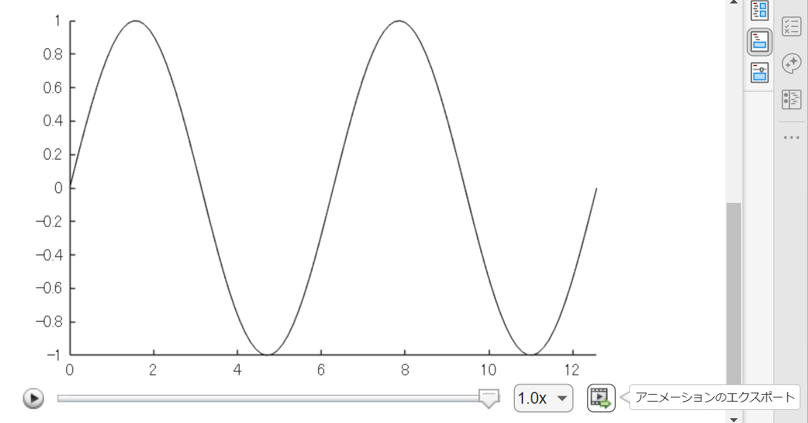
Livescript 上で for ループ内で描画を編集させて描いた動画は「アニメーションのエクスポート」から動画ファイルに出力するのが一番簡単ですね。再生速度やら細かい設定ができない点は要注意。
方法②
exportgraphics 関数で "Append" オプション指定で実現できるようになった(R2022a から)のでこれも便利ですね。
N = 100;
x = linspace(0,4*pi,N);
y = sin(x);
filename = 'animation_sample.gif'; % Specify the output file name
if exist(filename,'file')
delete(filename)
end
h = animatedline;
axis([0,4*pi,-1,1]) % x軸の表示範囲を固定
for k = 1:length(x)
addpoints(h,x(k),y(k)); % ループでデータを追加
exportgraphics(gca,filename,"Append",true)
end
方法③
R2021b 以前のバージョンだとこんな感じ。
各ループで画面キャプチャして、imwrite で動画ファイルにフレーム追加していくイメージです。"DelayTime" を使って細かい指定ができるので、必要に応じて今でも利用します。
for k = 1:length(x)
addpoints(h,x(k),y(k)); % ループでデータを追加
drawnow % グラフアップデート
frame = getframe(gcf); % Figure 画面をムービーフレーム(構造体)としてキャプチャ
tmp = frame2im(frame); % 画像に変更
[A,map] = rgb2ind(tmp,256); % RGB -> インデックス画像に
if k == 1 % 新規 gif ファイル作成
imwrite(A,map,filename,'gif','LoopCount',Inf,'DelayTime',0.2);
else % 以降、画像をアペンド
imwrite(A,map,filename,'gif','WriteMode','append','DelayTime',0.2);
end
end
I saw this on Reddit and thought of the past mini-hack contests. We have a few folks here who can do something similar with MATLAB.
これからは生成AIでコードを1から書くという事が減ってくるのかと思いますが,皆さんがMATLABのコードを書く時に意識しているご自身のルールのようなものがあれば教えてください.
MATLAB言語は柔軟に書けますが,自然と個人個人のルールというものが出来上がってきているのでは,と思います.
私はParameter, Valueペアの引数がある関数はそれぞれのペアを新しい行に書く,というのをよくやります.
h = plot(x, y, "ro-", ...
"LineWidth", 2, ...
"MarkerSize", 10, ...
"MarkerFaceColor", "g");
Parameter=Valueでも同じです.
h = plot(x, y, "ro-", ...
LineWidth = 2, ...
MarkerSize = 10, ...
MarkerFaceColor = "g");
また,一時期は "=" を揃えることもやってました(今はやってませんが).
h = plot(x, y, "ro-", ...
LineWidth = 2, ...
MarkerSize = 10, ...
MarkerFaceColor = "g");
皆さんにはどのようなルールがありますか?
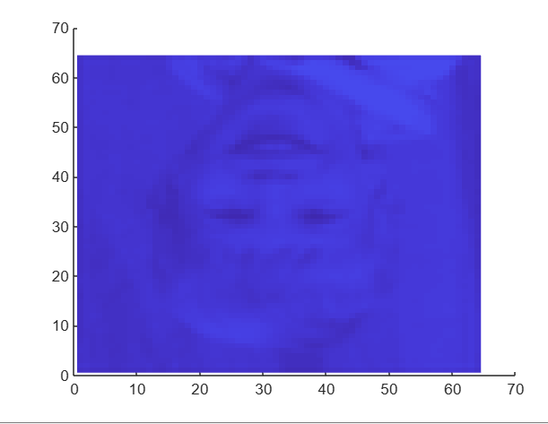
I had an error in the web version Matlab, so I exited and came back in, and this boy was plotted.
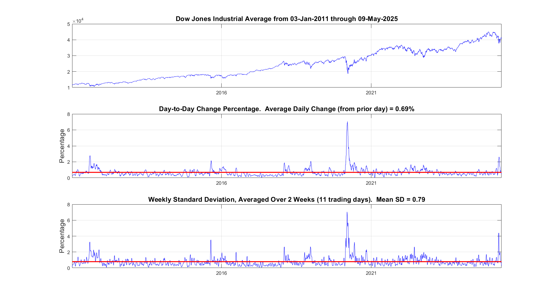
It seems like the financial news is always saying the stock market is especially volatile now. But is it really? This code will show you the daily variation from the prior day. You can see that the average daily change from one day to the next is 0.69%. So any change in the stock market from the prior day less than about 0.7% or 1% is just normal "noise"/typical variation. You can modify the code to adjust the starting date for the analysis. Data file (Excel workbook) is attached (hopefully - I attached it twice but it's not showing up yet).
% Program to plot the Dow Jones Industrial Average from 1928 to May 2025, and compute the standard deviation.
% Data available for download at https://finance.yahoo.com/quote/%5EDJI/history?p=%5EDJI
% Just set the Time Period, then find and click the download link, but you ned a paid version of Yahoo.
%
% If you have a subscription for Microsoft Office 365, you can also get historical stock prices.
% Reference: https://support.microsoft.com/en-us/office/stockhistory-function-1ac8b5b3-5f62-4d94-8ab8-7504ec7239a8#:~:text=The%20STOCKHISTORY%20function%20retrieves%20historical,Microsoft%20365%20Business%20Premium%20subscription.
% For example put this in an Excel Cell
% =STOCKHISTORY("^DJI", "1/1/2000", "5/10/2025", 0, 1, 0, 1,2,3,4, 5)
% and it will fill out a table in Excel
%====================================================================================================================
clc; % Clear the command window.
close all; % Close all figures (except those of imtool.)
imtool close all; % Close all imtool figures if you have the Image Processing Toolbox.
clear; % Erase all existing variables. Or clearvars if you want.
workspace; % Make sure the workspace panel is showing.
format long g;
format compact;
fontSize = 14;
filename = 'Dow Jones Industrial Index.xlsx';
data = readtable(filename);
% Date,Close,Open,High,Low,Volume
dates = data.Date;
closing = data.Close;
volume = data.Volume;
% Define start date and stop date
startDate = datetime(2011,1,1)
stopDate = dates(end)
selectedDates = dates > startDate;
% Extract those dates:
dates = dates(selectedDates);
closing = closing(selectedDates);
volume = volume(selectedDates);
% Plot Volume
hFigVolume = figure('Name', 'Daily Volume');
plot(dates, volume, 'b-');
grid on;
xticks(startDate:calendarDuration(5,0,0):stopDate)
title('Dow Jones Industrial Average Volume', 'FontSize', fontSize);
hFig = figure('Name', 'Daily Standard Deviation');
subplot(3, 1, 1);
plot(dates, closing, 'b-');
xticks(startDate:calendarDuration(5,0,0):stopDate)
drawnow;
grid on;
caption = sprintf('Dow Jones Industrial Average from %s through %s', dates(1), dates(end));
title(caption, 'FontSize', fontSize);
% Get the average change from one trading day to the next.
diffs = 100 * abs(closing(2:end) - closing(1:end-1)) ./ closing(1:end-1);
subplot(3, 1, 2);
averageDailyChange = mean(diffs)
% Looks pretty noisy so let's smooth it for a nicer display.
numWeeks = 4;
diffs = sgolayfilt(diffs, 2, 5*numWeeks+1);
plot(dates(2:end), diffs, 'b-');
grid on;
xticks(startDate:calendarDuration(5,0,0):stopDate)
hold on;
line(xlim, [averageDailyChange, averageDailyChange], 'Color', 'r', 'LineWidth', 2);
ylabel('Percentage', 'FontSize', fontSize);
caption = sprintf('Day-to-Day Change Percentage. Average Daily Change (from prior day) = %.2f%%', averageDailyChange);
title(caption, 'FontSize', fontSize);
drawnow;
% Get the stddev over a 5 trading day window.
sd = stdfilt(closing, ones(5, 1));
% Get it relative to the magnitude.
sd = sd ./ closing * 100;
averageVariation = mean(sd)
numWeeks = 2;
% Looks pretty noisy so let's smooth it for a nicer display.
sd = sgolayfilt(sd, 2, 5*numWeeks+1);
% Plot it.
subplot(3, 1, 3);
plot(dates, sd, 'b-');
grid on;
xticks(startDate:calendarDuration(5,0,0):stopDate)
hold on;
line(xlim, [averageVariation, averageVariation], 'Color', 'r', 'LineWidth', 2);
ylabel('Percentage', 'FontSize', fontSize);
caption = sprintf('Weekly Standard Deviation, Averaged Over %d Weeks (%d trading days). Mean SD = %.2f', ...
numWeeks, 5*numWeeks+1, averageVariation);
title(caption, 'FontSize', fontSize);
% Maximize figure window.
g = gcf;
g.WindowState = 'maximized';
昨日 5/29 にお台場で MATLAB EXPO が開催されました。ご参加くださった方々ありがとうございました!
私は AI 関連のデモ展示で解説員としても立っておりましたが、立ち寄ってくださる方が絶えず、ずっと喋り続けてました。また、講演後に「さっきのすごくね?」という会話が漏れ聞こえてきたのがハイライト。
参加されたみなさま、印象に残ったこと・気になった講演・ポスター・デモ・新機能等あったら教えてください!(次回に向けて運営面での感想も)
以前のEXPOでも参加・聴講したことがある
67%
知り合いから聞いた
0%
MathWorksからのプロモーション,EXPOサイトで知った
0%
今年のEXPO会場でたまたま見かけた
0%
ライトニングトークって何?
33%
3 票
I like this problem by James and have solved it in several ways. A solution by Natalie impressed me and introduced me to a new function conv2. However, it occured to me that the numerous test for the problem only cover cases of square matrices. My original solutions, and Natalie's, did niot work on rectangular matrices. I have now produced a solution which works on rectangular matrices. Thanks for this thought provoking problem James.
I wanted to turn a Markdown nested list of text labels:
- A
- B
- C
- D
- G
- H
- E
- F
- Q
into a directed graph, like this:

Here is my blog post with some related tips for doing this, including text I/O, text processing with patterns, and directed graph operations and visualization.