LiDAR データからのマップの作成

この例では次を使用します。

この例では、慣性測定装置 (IMU) の読み取り値を利用し、車両に取り付けられたセンサーからの 3 次元 LiDAR データを処理して、徐々にマップを作成する方法を説明します。このようなマップは、車両ナビゲーションの経路計画に役立ち、位置推定にも使用できます。生成されたマップを評価するために、この例では車両の軌跡を全地球測位システム (GPS) と比較する方法も説明します。

概要

高精細 (HD) マップは、数センチメートル以内の精度で道路の正確なジオメトリを提供する地図作成サービスです。この精度の高さにより、HD マップは位置推定やナビゲーションなどの自動運転ワークフローに最適です。このような HD マップは、高精度な GPS や IMU センサーを併用し、3 次元 LiDAR スキャンからマップを作成することによって生成されます。これを使用して、車両を数センチメートル以内の精度で位置推定できます。この例では、こうしたシステムをビルドするために必要な機能の一部を実装します。

この例では、次を行う方法を学びます。

記録された走行データの読み込み、調査、および可視化
LiDAR スキャンを使用したマップの作成
IMU の読み取り値を使用したマップの改善

記録された走行データの読み込みと調査

この例で使用するデータはこの GitHub® リポジトリのものであり、約 100 秒間の LiDAR、GPS、および IMU のデータです。データは MAT ファイル形式で保存されており、それぞれにtimetableが含まれています。リポジトリから MAT ファイルをダウンロードし、MATLAB® ワークスペースに読み込みます。

メモ: このダウンロードは数分かかることがあります。

baseDownloadURL = 'https://github.com/mathworks/udacity-self-driving-data-subset/raw/master/drive_segment_11_18_16/';
dataFolder      = fullfile(tempdir, 'drive_segment_11_18_16', filesep);
options         = weboptions('Timeout', Inf);

lidarFileName = dataFolder + "lidarPointClouds.mat";
imuFileName   = dataFolder + "imuOrientations.mat";
gpsFileName   = dataFolder + "gpsSequence.mat";

folderExists  = exist(dataFolder, 'dir');
matfilesExist = exist(lidarFileName, 'file') && exist(imuFileName, 'file') ...
    && exist(gpsFileName, 'file');

if ~folderExists
    mkdir(dataFolder);
end

if ~matfilesExist
    disp('Downloading lidarPointClouds.mat (613 MB)...')
    websave(lidarFileName, baseDownloadURL + "lidarPointClouds.mat", options);

    disp('Downloading imuOrientations.mat (1.2 MB)...')
    websave(imuFileName, baseDownloadURL + "imuOrientations.mat", options);

    disp('Downloading gpsSequence.mat (3 KB)...')
    websave(gpsFileName, baseDownloadURL + "gpsSequence.mat", options);
end

Downloading lidarPointClouds.mat (613 MB)...
Downloading imuOrientations.mat (1.2 MB)...
Downloading gpsSequence.mat (3 KB)...

まず、Velodyne® HDL32E LiDAR から保存された点群データを読み込みます。LiDAR データの各スキャンが、pointCloudオブジェクトを使用して 3 次元点群として格納されます。このオブジェクトは、K-d 木のデータ構造を使用して内部的にデータを整理し、探索の高速化を図ります。各 LiDAR スキャンに関連付けられたタイムスタンプは、timetable の変数 Time に記録されます。

% Load lidar data from MAT-file
data = load(lidarFileName);
lidarPointClouds = data.lidarPointClouds;

% Display first few rows of lidar data
head(lidarPointClouds)

        Time           PointCloud  
    _____________    ______________

    23:46:10.5115    1×1 pointCloud
    23:46:10.6115    1×1 pointCloud
    23:46:10.7116    1×1 pointCloud
    23:46:10.8117    1×1 pointCloud
    23:46:10.9118    1×1 pointCloud
    23:46:11.0119    1×1 pointCloud
    23:46:11.1120    1×1 pointCloud
    23:46:11.2120    1×1 pointCloud

GPS のデータを MAT ファイルから読み込みます。車両の GPS デバイスによって記録された地理座標が、timetable の変数 Latitude、Longitude、および Altitude を使用して格納されます。

% Load GPS sequence from MAT-file
data = load(gpsFileName);
gpsSequence = data.gpsSequence;

% Display first few rows of GPS data
head(gpsSequence)

        Time         Latitude    Longitude    Altitude
    _____________    ________    _________    ________

    23:46:11.4563      37.4       -122.11      -42.5  
    23:46:12.4563      37.4       -122.11      -42.5  
    23:46:13.4565      37.4       -122.11      -42.5  
    23:46:14.4455      37.4       -122.11      -42.5  
    23:46:15.4455      37.4       -122.11      -42.5  
    23:46:16.4567      37.4       -122.11      -42.5  
    23:46:17.4573      37.4       -122.11      -42.5  
    23:46:18.4656      37.4       -122.11      -42.5

IMU のデータを MAT ファイルから読み込みます。IMU は一般的に、車両の動きに関する情報を報告する個々のセンサーで構成されています。加速度計、ジャイロスコープ、磁力計など、複数のセンサーが組み合わせられています。変数 Orientation は、報告された IMU センサーの向きを格納します。これらの読み取り値は四元数として報告されます。各読み取り値は、4 つの四元数部分を含む 1 行 4 列のベクトルとして指定されます。1 行 4 列のベクトルをquaternion (Automated Driving Toolbox)オブジェクトに変換します。

% Load IMU recordings from MAT-file
data = load(imuFileName);
imuOrientations = data.imuOrientations;

% Convert IMU recordings to quaternion type
imuOrientations = convertvars(imuOrientations, 'Orientation', 'quaternion');

% Display first few rows of IMU data
head(imuOrientations)

        Time          Orientation  
    _____________    ______________

    23:46:11.4570    1×1 quaternion
    23:46:11.4605    1×1 quaternion
    23:46:11.4620    1×1 quaternion
    23:46:11.4655    1×1 quaternion
    23:46:11.4670    1×1 quaternion
    23:46:11.4705    1×1 quaternion
    23:46:11.4720    1×1 quaternion
    23:46:11.4755    1×1 quaternion

センサーの読み取り値がどのように入ってくるかを理解するために、センサーごとに、フレームのおおよそのdurationを計算します。

lidarFrameDuration = median(diff(lidarPointClouds.Time));
gpsFrameDuration   = median(diff(gpsSequence.Time));
imuFrameDuration   = median(diff(imuOrientations.Time));

% Adjust display format to seconds
lidarFrameDuration.Format = 's';
gpsFrameDuration.Format   = 's';
imuFrameDuration.Format   = 's';

% Compute frame rates
lidarRate = 1/seconds(lidarFrameDuration);
gpsRate   = 1/seconds(gpsFrameDuration);
imuRate   = 1/seconds(imuFrameDuration);

% Display frame durations and rates
fprintf('Lidar: %s, %3.1f Hz\n', char(lidarFrameDuration), lidarRate);
fprintf('GPS  : %s, %3.1f Hz\n', char(gpsFrameDuration), gpsRate);
fprintf('IMU  : %s, %3.1f Hz\n', char(imuFrameDuration), imuRate);

Lidar: 0.10008 sec, 10.0 Hz
GPS  : 1.0001 sec, 1.0 Hz
IMU  : 0.002493 sec, 401.1 Hz

GPS センサーが最も遅く、約 1 Hz のレートで実行されています。次に遅いのが LiDAR でレートは約 10 Hz、次が IMU でレートは約 400 Hz で実行されています。

走行データの可視化

シーンの内容を理解するため、ストリーミングプレーヤーを使用して記録データを可視化します。GPS の読み取り値を可視化するには、geoplayer (Automated Driving Toolbox)を使用します。LiDAR の読み取り値を可視化するには、pcplayerを使用します。

% Create a geoplayer to visualize streaming geographic coordinates
latCenter = gpsSequence.Latitude(1);
lonCenter = gpsSequence.Longitude(1);
zoomLevel = 17;

gpsPlayer = geoplayer(latCenter, lonCenter, zoomLevel);

% Plot the full route
plotRoute(gpsPlayer, gpsSequence.Latitude, gpsSequence.Longitude);

% Determine limits for the player
xlimits = [-45 45]; % meters
ylimits = [-45 45];
zlimits = [-10 20];

% Create a pcplayer to visualize streaming point clouds from lidar sensor
lidarPlayer = pcplayer(xlimits, ylimits, zlimits);

% Customize player axes labels
xlabel(lidarPlayer.Axes, 'X (m)')
ylabel(lidarPlayer.Axes, 'Y (m)')
zlabel(lidarPlayer.Axes, 'Z (m)')

title(lidarPlayer.Axes, 'Lidar Sensor Data')

% Align players on screen
helperAlignPlayers({gpsPlayer, lidarPlayer});

% Outer loop over GPS readings (slower signal)
for g = 1 : height(gpsSequence)-1

    % Extract geographic coordinates from timetable
    latitude  = gpsSequence.Latitude(g);
    longitude = gpsSequence.Longitude(g);

    % Update current position in GPS display
    plotPosition(gpsPlayer, latitude, longitude);

    % Compute the time span between the current and next GPS reading
    timeSpan = timerange(gpsSequence.Time(g), gpsSequence.Time(g+1));

    % Extract the lidar frames recorded during this time span
    lidarFrames = lidarPointClouds(timeSpan, :);

    % Inner loop over lidar readings (faster signal)
    for l = 1 : height(lidarFrames)

        % Extract point cloud
        ptCloud = lidarFrames.PointCloud(l);

        % Update lidar display
        view(lidarPlayer, ptCloud);

        % Pause to slow down the display
        pause(0.01)
    end
end

記録された LiDAR データを使用したマップの作成

LiDAR は強力なセンサーであり、他のセンサーが使えない厳しい環境での認識に使用できます。車両の環境について、詳細な 360 度全体の視野を提供します。

% Hide players
hide(gpsPlayer)
hide(lidarPlayer)

% Select a frame of lidar data to demonstrate registration workflow
frameNum = 600;
ptCloud = lidarPointClouds.PointCloud(frameNum);

% Display and rotate ego view to show lidar data
helperVisualizeEgoView(ptCloud);

LiDAR を使用して、都市全体の HD マップなど、センチメートル級の精度の HD マップを作成できます。これらのマップは、後で車両内からの位置推定に使用できます。このようなマップを作成するための一般的なアプローチは、走行車両から取得した連続的な LiDAR スキャンを整列させて、1 つの大きな点群に集約することです。この例の残りの部分では、このマップの作成のアプローチについて検討します。

LiDAR スキャンを整列させる: 反復最近接点 (ICP) アルゴリズムや正規分布変換 (NDT) アルゴリズムなどの点群レジストレーションの手法を使用して、連続的な LiDAR スキャンを整列させます。各アルゴリズムの詳細については、pcregistericpおよびpcregisterndtを参照してください。この例では、Generalized-ICP (G-ICP) アルゴリズムを使用します。関数 pcregistericp は、基準点群に対して移動点群を整列させる剛体変換を返します。これらの変換を連続して構成することにより、各点群は最初の点群の基準座標系に変換されます。
整列したスキャンを組み合わせる: 新しい点群スキャンのレジストレーションが行われ、変換されて最初の点群の基準フレームに戻ったら、pcmergeを使用して、その点群を最初の点群とマージできます。

まず、隣接する LiDAR スキャンに対応する 2 つの点群を取得します。処理を高速化するため、そしてスキャン間に十分な動きを蓄積するために、10 スキャンごとに使用します。

skipFrames = 10;
frameNum   = 100;

fixed  = lidarPointClouds.PointCloud(frameNum);
moving = lidarPointClouds.PointCloud(frameNum + skipFrames);

レジストレーションの前に点群をダウンサンプリングします。ダウンサンプリングにより、レジストレーション精度とアルゴリズム速度の両方が向上します。

downsampleGridStep = 0.2;
fixedDownsampled  = pcdownsample(fixed, 'gridAverage', downsampleGridStep);
movingDownsampled = pcdownsample(moving, 'gridAverage', downsampleGridStep);

点群を前処理した後、Generalized-ICP アルゴリズムを使用して点群をレジストレーションします。これは、pcregistericpで名前と値の引数 Metric を 'planeToPlane' に設定することで使用できます。レジストレーションの前と後の整列を可視化します。

regInlierRatio = 0.35;
tform = pcregistericp(movingDownsampled, fixedDownsampled, 'Metric', 'planeToPlane', ...
    'InlierRatio', regInlierRatio);

movingReg = pctransform(movingDownsampled, tform);

% Visualize alignment in top-view before and after registration
hFigAlign = figure;

subplot(121)
pcshowpair(movingDownsampled, fixedDownsampled)
title('Before Registration')
view(2)

subplot(122)
pcshowpair(movingReg, fixedDownsampled)
title('After Registration')
view(2)

helperMakeFigurePublishFriendly(hFigAlign);

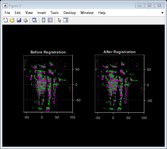
レジストレーション後の点群はよく整列されていることがわかります。点群はかなり整列されていますが、まだ完全ではありません。

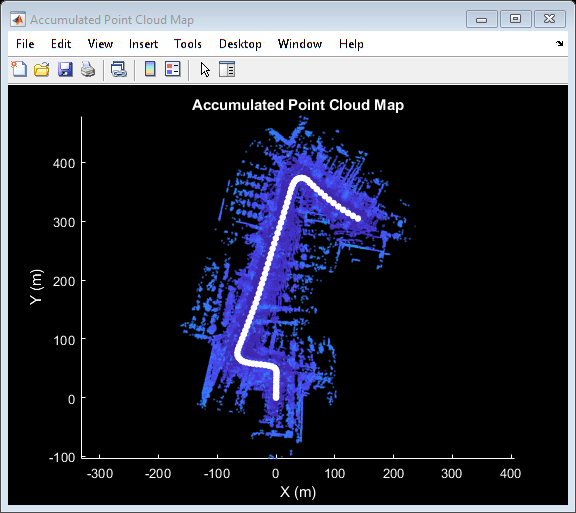
次に、pcmerge を使用して点群をマージします。

mergeGridStep = 0.5;
ptCloudAccum = pcmerge(fixedDownsampled, movingReg, mergeGridStep);

hFigAccum = figure;
pcshow(ptCloudAccum)
title('Accumulated Point Cloud')
view(2)

helperMakeFigurePublishFriendly(hFigAccum);

点群のペアを 1 つ処理するパイプラインが理解できたところで、記録データのシーケンス全体に対するループでこれをまとめて行います。helperLidarMapBuilder クラスにこのすべてがまとめられています。このクラスの updateMap メソッドは、新しい点群を受け取り、先ほど説明した次のステップを実行します。

点群をダウンサンプリングします。
前回の点群を今回の点群とマージするために必要な剛体変換を推定します。
点群を変換して、最初のフレームに戻します。
この点群を、蓄積された点群マップとマージします。

また、updateMap メソッドは初期変換推定も受け取ります。これは、レジストレーションの初期化に使用されます。適切な初期化により、レジストレーションの結果を大幅に向上させることができます。逆に、不適切な初期化は、レジストレーションに悪影響を与える可能性があります。適切な初期化を行うことで、アルゴリズムの実行時間を改善することもできます。

レジストレーションの初期推定を行うには、等速度の仮定を使用するのが一般的なアプローチです。前回の反復の変換を初期推定として使用します。

updateDisplay メソッドは、2 次元上面図のストリーミング点群表示の作成と更新も行います。

% Create a map builder object
mapBuilder = helperLidarMapBuilder('DownsampleGridStep', downsampleGridStep);

% Set random number seed
rng(0);

closeDisplay = false;
numFrames    = height(lidarPointClouds);

tform = rigidtform3d;
for n = 1 : skipFrames : numFrames - skipFrames + 1

    % Get the nth point cloud
    ptCloud = lidarPointClouds.PointCloud(n);

    % Use transformation from previous iteration as initial estimate for
    % current iteration of point cloud registration. (constant velocity)
    initTform = tform;

    % Update map using the point cloud
    tform = updateMap(mapBuilder, ptCloud, initTform);

    % Update map display
    updateDisplay(mapBuilder, closeDisplay);
end

点群レジストレーションのみで、車両がたどった環境のマップを作成します。マップは局所的には一貫性があるように見えますが、シーケンス全体を通して大幅なドリフトが生じている場合があります。

記録された GPS の読み取り値をグラウンドトゥルースの軌跡として使用し、作成されたマップの質を視覚的に評価します。まず、GPS の読み取り値 (緯度、経度、高度) をローカル座標系に変換します。シーケンスにおける最初の点群の原点と一致するローカル座標系を選択します。この変換は、次の 2 つの変換を使用して計算されます。

関数latlon2local (Automated Driving Toolbox)を使用して、GPS 座標をローカルの直交 East-North-Up 座標に変換します。軌跡の始点の GPS 位置を基準点として使用し、ローカル X、Y、Z 座標系の原点を定義します。
ローカル座標系が最初の LiDAR センサー座標と合うよう、直交座標を回転させます。車両上の LiDAR と GPS の厳密な取り付け構成は不明なので、推定します。

% Select reference point as first GPS reading
origin = [gpsSequence.Latitude(1), gpsSequence.Longitude(1), gpsSequence.Altitude(1)];

% Convert GPS readings to a local East-North-Up coordinate system
[xEast, yNorth, zUp] = latlon2local(gpsSequence.Latitude, gpsSequence.Longitude, ...
    gpsSequence.Altitude, origin);

% Estimate rough orientation at start of trajectory to align local ENU
% system with lidar coordinate system
theta = median(atan2d(yNorth(1:15), xEast(1:15)));

R = [ cosd(90-theta) sind(90-theta) 0;
     -sind(90-theta) cosd(90-theta) 0;
     0               0              1];

% Rotate ENU coordinates to align with lidar coordinate system
groundTruthTrajectory = [xEast, yNorth, zUp] * R;

作成したマップにグラウンドトゥルースの軌跡を重ね合わせます。

hold(mapBuilder.Axes, 'on')
scatter(mapBuilder.Axes, groundTruthTrajectory(:,1), groundTruthTrajectory(:,2), ...
    'green', 'filled');

helperAddLegend(mapBuilder.Axes, ...
    {'Map Points', 'Estimated Trajectory', 'Ground Truth Trajectory'});

軌跡間の平方根平均二乗誤差 (rmse) を計算して、推定された軌跡とグラウンドトゥルースの軌跡を比較します。

estimatedTrajectory = vertcat(mapBuilder.ViewSet.Views.AbsolutePose.Translation);
accuracyMetric = rmse(groundTruthTrajectory, estimatedTrajectory, 'all');

disp(['rmse between ground truth and estimated trajectory: ' num2str(accuracyMetric)])

rmse between ground truth and estimated trajectory: 9.773

最初のターンの後、推定軌跡はグラウンドトゥルースの軌跡から大幅に逸脱します。点群レジストレーションのみを使用して推定した軌跡は、次のいくつかの理由でドリフトする可能性があります。

センサーからのスキャンにノイズが多く、十分なオーバーラップがない
十分に強い特徴がない (近接する長い道路など)
特に大きく回転している場合に、初期変換が不正確

% Close map display
updateDisplay(mapBuilder, true);

IMU の向きを使用した作成されたマップの改善

IMU はプラットフォーム上に取り付けられた電子デバイスです。IMU には複数のセンサーが含まれており、これらが車両の動きに関する各種の情報を報告します。一般的な IMU には、加速度計、ジャイロスコープ、および磁力計が組み込まれています。IMU により、信頼性の高い向きの測定ができます。

IMU の読み取り値を使用して、レジストレーションのための初期推定を向上させます。この例で使用する、IMU から報告されたセンサーの読み取り値は、デバイス上でフィルター済みです。

% Reset the map builder to clear previously built map
reset(mapBuilder);

% Set random number seed
rng(0);

initTform = rigidtform3d;
for n = 1 : skipFrames : numFrames - skipFrames + 1

    % Get the nth point cloud
    ptCloud = lidarPointClouds.PointCloud(n);

    if n > 1
        % Since IMU sensor reports readings at a much faster rate, gather
        % IMU readings reported since the last lidar scan.
        prevTime = lidarPointClouds.Time(n - skipFrames);
        currTime = lidarPointClouds.Time(n);
        timeSinceScan = timerange(prevTime, currTime);

        imuReadings = imuOrientations(timeSinceScan, 'Orientation');

        % Form an initial estimate using IMU readings
        initTform = helperComputeInitialEstimateFromIMU(imuReadings, tform);
    end

    % Update map using the point cloud
    tform = updateMap(mapBuilder, ptCloud, initTform);

    % Update map display
    updateDisplay(mapBuilder, closeDisplay);
end

% Superimpose ground truth trajectory on new map
hold(mapBuilder.Axes, 'on')
scatter(mapBuilder.Axes, groundTruthTrajectory(:,1), groundTruthTrajectory(:,2), ...
    'green', 'filled');

helperAddLegend(mapBuilder.Axes, ...
    {'Map Points', 'Estimated Trajectory', 'Ground Truth Trajectory'});

% Capture snapshot for publishing
snapnow;

% Close open figures
close([hFigAlign, hFigAccum]);
updateDisplay(mapBuilder, true);

% Compare the trajectory estimated using the IMU orientation with the
% ground truth trajectory
estimatedTrajectory = vertcat(mapBuilder.ViewSet.Views.AbsolutePose.Translation);
accuracyMetricWithIMU = rmse(groundTruthTrajectory, estimatedTrajectory, 'all');

disp(['rmse between ground truth and trajectory estimated using IMU orientation: ' num2str(accuracyMetricWithIMU)])

rmse between ground truth and trajectory estimated using IMU orientation: 3.4613

IMU による向きの推定を使用したことでレジストレーションが大幅に改善し、より近似した、ドリフトの小さい軌跡が得られました。

サポート関数

helperAlignPlayers は、ストリーミングプレーヤーの cell 配列を整列し、画面の左から右へ並べます。

function helperAlignPlayers(players)

validateattributes(players, {'cell'}, {'vector'});

hasAxes = cellfun(@(p)isprop(p,'Axes'),players,'UniformOutput', true);
if ~all(hasAxes)
    error('Expected all viewers to have an Axes property');
end

screenSize   = get(groot, 'ScreenSize');
screenMargin = [50, 100];

playerSizes = cellfun(@getPlayerSize, players, 'UniformOutput', false);
playerSizes = cell2mat(playerSizes);

maxHeightInSet = max(playerSizes(1:3:end));

% Arrange players vertically so that the tallest player is 100 pixels from
% the top.
location = round([screenMargin(1), screenSize(4)-screenMargin(2)-maxHeightInSet]);
for n = 1 : numel(players)
    player = players{n};

    hFig = ancestor(player.Axes, 'figure');
    hFig.OuterPosition(1:2) = location;

    % Set up next location by going right
    location = location + [50+hFig.OuterPosition(3), 0];
end

    function sz = getPlayerSize(viewer)

        % Get the parent figure container
        h = ancestor(viewer.Axes, 'figure');

        sz = h.OuterPosition(3:4);
    end
end

helperVisualizeEgoView は、中心点回りに回転させることで、点群データを自車視点で可視化します。

function player = helperVisualizeEgoView(ptCloud)

% Create a pcplayer object
xlimits = ptCloud.XLimits;
ylimits = ptCloud.YLimits;
zlimits = ptCloud.ZLimits;

player = pcplayer(xlimits, ylimits, zlimits);

% Turn off axes lines
axis(player.Axes, 'off');

% Set up camera to show ego view
camproj(player.Axes, 'perspective');
camva(player.Axes, 90);
campos(player.Axes, [0 0 0]);
camtarget(player.Axes, [-1 0 0]);

% Set up a transformation to rotate by 5 degrees
theta = 5;

eulerAngles = [0 0 theta];
translation = [0 0 0];
rotateByTheta = rigidtform3d(eulerAngles, translation);

for n = 0 : theta : 359
    % Rotate point cloud by theta
    ptCloud = pctransform(ptCloud, rotateByTheta);

    % Display point cloud
    view(player, ptCloud);

    pause(0.05)
end
end

helperComputeInitialEstimateFromIMU は、IMU の向きの読み取り値と前回推定した変換を使用して、レジストレーションのための初期変換を推定します。

function tform = helperComputeInitialEstimateFromIMU(imuReadings, prevTform)

% Initialize transformation using previously estimated transform
tform = prevTform;

% If no IMU readings are available, return
if height(imuReadings) <= 1
    return;
end

% IMU orientation readings are reported as quaternions representing the
% rotational offset to the body frame. Compute the orientation change
% between the first and last reported IMU orientations during the interval
% of the lidar scan.
q1 = imuReadings.Orientation(1);
q2 = imuReadings.Orientation(end);

% Compute rotational offset between first and last IMU reading by
%   - Rotating from q2 frame to body frame
%   - Rotating from body frame to q1 frame
q = q1 * conj(q2);

% Convert to Euler angles
yawPitchRoll = euler(q, 'ZYX', 'point');

% Discard pitch and roll angle estimates. Use only heading angle estimate
% from IMU orientation.
yawPitchRoll(2:3) = 0;

% Convert back to rotation matrix
q = quaternion(yawPitchRoll, 'euler', 'ZYX', 'point');
tform.R = rotmat(q, 'point');
end

helperAddLegend は、座標軸に凡例を追加します。

function helperAddLegend(hAx, labels)

% Add a legend to the axes
hLegend = legend(hAx, labels{:});

% Set text color and font weight
hLegend.TextColor  = [1 1 1];
hLegend.FontWeight = 'bold';
end

helperMakeFigurePublishFriendly は、publish で取得するスクリーンショットが適切になるよう、図を調整します。

function helperMakeFigurePublishFriendly(hFig)

if ~isempty(hFig) && isvalid(hFig)
    hFig.HandleVisibility = 'callback';
end

end

参考

関数

pcmerge | pcregistericp | pcregisterndt

オブジェクト

pcplayer | geoplayer (Automated Driving Toolbox) | pointCloud

外部の Web サイト

Udacity Self-Driving Car Data Subset (MathWorks GitHub リポジトリ)