R-CNN 深層学習を使用したオブジェクト検出器の学習

この例では次を使用します。

この例では、深層学習と R-CNN (Regions with Convolutional Neural Networks) を使用して、オブジェクト検出器に学習させる方法を説明します。

概要

この例では、一時停止標識を検出するために R-CNN オブジェクト検出器に学習させる方法を説明します。R-CNN はオブジェクト検出フレームワークで、畳み込みニューラルネットワーク (CNN) を使用してイメージ内のイメージ領域を分類します [1]。R-CNN では、スライディングウィンドウを使用して領域が 1 つずつ分類されるのではなく、オブジェクトが含まれる可能性が高い領域のみが処理されます。これにより CNN の実行時に発生する計算コストが大幅に減少します。

R-CNN の一時停止標識検出器に学習させる方法を説明するために、この例では、深層学習の用途でよく使用される転移学習のワークフローに沿っています。転移学習では、ImageNet [2] などの大規模なイメージコレクションで学習済みのネットワークが、新しい分類タスクや検出タスクを解決するための開始点として使用されます。この方法の利点は、事前学習済みネットワークが既にイメージの特徴を十分学習しており、これらの特徴をさまざまなイメージに適用できることです。この学習内容は、ネットワークを微調整することによって新しいタスクに転用できます。ネットワークの微調整は、重みを少し調整することによって行います。つまり、元のタスクで学習済みの特徴表現を新しいタスクに合わせてわずかに調整します。

転移学習には、学習に必要なイメージの数が少なくて済み、学習時間が短縮されるというメリットがあります。これらのメリットについて説明するために、この例では転移学習のワークフローを使用して一時停止標識検出器に学習させます。まず、50,000 個の学習イメージが含まれる CIFAR-10 データセットを使用して、CNN に事前学習させます。その後、学習イメージを 41 個だけ使用して、この事前学習済みの CNN を一時停止標識検出用に微調整します。事前学習済みの CNN を使用しない場合、より多くのイメージを使用して一時停止標識検出器に学習させる必要があります。

メモ: この例には、Computer Vision Toolbox™、Image Processing Toolbox™、Deep Learning Toolbox™ および Statistics and Machine Learning Toolbox™ が必要です。

この例を実行するには、CUDA 対応 NVIDIA™ GPU の使用が強く推奨されます。GPU を使用するには Parallel Computing Toolbox™ が必要です。サポートされる Compute Capability の詳細については、GPU 計算の要件 (Parallel Computing Toolbox)を参照してください。

CIFAR-10 イメージデータのダウンロード

CIFAR-10 データセット [3] をダウンロードします。このデータセットには、CNN に学習させるために使用する 50,000 個の学習イメージが含まれています。

CIFAR-10 データを一時ディレクトリにダウンロードします。

cifar10Data = tempdir;

url = 'https://www.cs.toronto.edu/~kriz/cifar-10-matlab.tar.gz';

helperCIFAR10Data.download(url,cifar10Data);

CIFAR-10 学習データとテストデータを読み込みます。

[trainingImages,trainingLabels,testImages,testLabels] = helperCIFAR10Data.load(cifar10Data);

それぞれのイメージは 32x32 RGB イメージで、50,000 個の学習サンプルがあります。

size(trainingImages)

ans = 1×4

          32          32           3       50000

CIFAR-10 には 10 個のイメージカテゴリがあります。イメージカテゴリを一覧表示します。

numImageCategories = 10;
categories(trainingLabels)

ans = 10×1 cell
    {'airplane'  }
    {'automobile'}
    {'bird'      }
    {'cat'       }
    {'deer'      }
    {'dog'       }
    {'frog'      }
    {'horse'     }
    {'ship'      }
    {'truck'     }

次のコードを使用すると、いくつかの学習イメージを表示できます。

figure
thumbnails = trainingImages(:,:,:,1:100);
montage(thumbnails)

畳み込みニューラルネットワーク (CNN) の作成

CNN は一連の層で構成されています。各層では特定の計算が定義されます。Deep Learning Toolbox™ は、CNN を層単位で簡単に設計する機能を提供します。この例では、次の層を使用して CNN を作成します。

imageInputLayer (Deep Learning Toolbox) - イメージ入力層
convolution2dLayer (Deep Learning Toolbox) - 畳み込みニューラルネットワーク用の 2 次元畳み込み層
reluLayer (Deep Learning Toolbox) - 正規化線形ユニット (ReLU) 層
maxPooling2dLayer (Deep Learning Toolbox) - 最大プーリング層
fullyConnectedLayer (Deep Learning Toolbox) - 全結合層
softmaxLayer (Deep Learning Toolbox) - ソフトマックス層
classificationLayer (Deep Learning Toolbox) - ニューラルネットワーク用の分類出力層

ここで定義するネットワークは、[4] で説明されているネットワークと同様に、imageInputLayer から始まります。入力層は、CNN が処理できるデータのタイプとサイズを定義します。この例では、CNN を使用して CIFAR-10 イメージ (32x32 RGB イメージ) を処理します。

% Create the image input layer for 32x32x3 CIFAR-10 images.
[height,width,numChannels, ~] = size(trainingImages);

imageSize = [height width numChannels];
inputLayer = imageInputLayer(imageSize)

inputLayer = 
  ImageInputLayer with properties:

                      Name: ''
                 InputSize: [32 32 3]
   Hyperparameters
          DataAugmentation: 'none'
             Normalization: 'zerocenter'
    NormalizationDimension: 'auto'
                      Mean: []

次に、ネットワークの中間層を定義します。中間層は、畳み込み層、ReLU (正規化線形ユニット) およびプーリング層のブロックの繰り返しで構成されています。これら 3 つの層が、畳み込みニューラルネットワークの中核となる基本ブロックを形成します。畳み込み層は、ネットワークの学習中に更新されるフィルターの一連の重みを定義します。ReLU 層は、ネットワークに非線形性を追加します。これにより、ネットワークでイメージピクセルをイメージのセマンティクスコンテンツにマッピングする非線形関数を近似できます。プーリング層は、ネットワークを流れるデータをダウンサンプリングします。多数の層があるネットワークでは、ネットワークでのデータのダウンサンプリングが早くなりすぎないように、プーリング層を慎重に使用してください。

% Convolutional layer parameters
filterSize = [5 5];
numFilters = 32;

middleLayers = [
    
% The first convolutional layer has a bank of 32 5x5x3 filters. A
% symmetric padding of 2 pixels is added to ensure that image borders
% are included in the processing. This is important to avoid
% information at the borders being washed away too early in the
% network.
convolution2dLayer(filterSize,numFilters,'Padding',2)

% Note that the third dimension of the filter can be omitted because it
% is automatically deduced based on the connectivity of the network. In
% this case because this layer follows the image layer, the third
% dimension must be 3 to match the number of channels in the input
% image.

% Next add the ReLU layer:
reluLayer()

% Follow it with a max pooling layer that has a 3x3 spatial pooling area
% and a stride of 2 pixels. This down-samples the data dimensions from
% 32x32 to 15x15.
maxPooling2dLayer(3,'Stride',2)

% Repeat the 3 core layers to complete the middle of the network.
convolution2dLayer(filterSize,numFilters,'Padding',2)
reluLayer()
maxPooling2dLayer(3, 'Stride',2)

convolution2dLayer(filterSize,2 * numFilters,'Padding',2)
reluLayer()
maxPooling2dLayer(3,'Stride',2)

]

middleLayers = 
  9x1 Layer array with layers:

     1   ''   Convolution   32 5x5 convolutions with stride [1  1] and padding [2  2  2  2]
     2   ''   ReLU          ReLU
     3   ''   Max Pooling   3x3 max pooling with stride [2  2] and padding [0  0  0  0]
     4   ''   Convolution   32 5x5 convolutions with stride [1  1] and padding [2  2  2  2]
     5   ''   ReLU          ReLU
     6   ''   Max Pooling   3x3 max pooling with stride [2  2] and padding [0  0  0  0]
     7   ''   Convolution   64 5x5 convolutions with stride [1  1] and padding [2  2  2  2]
     8   ''   ReLU          ReLU
     9   ''   Max Pooling   3x3 max pooling with stride [2  2] and padding [0  0  0  0]

これら 3 つの基本層を繰り返すことで、より深いネットワークを作成できます。ただし、プーリング層の数を減らして、データが途中でダウンサンプリングされることを防いでください。ネットワークでダウンサンプリングが早く行われると、学習に役立つイメージ情報が破棄されます。

CNN の最終層は、通常、全結合層とソフトマックス損失層で構成されます。

finalLayers = [
    
% Add a fully connected layer with 64 output neurons. The output size of
% this layer will be an array with a length of 64.
fullyConnectedLayer(64)

% Add an ReLU non-linearity.
reluLayer

% Add the last fully connected layer. At this point, the network must
% produce 10 signals that can be used to measure whether the input image
% belongs to one category or another. This measurement is made using the
% subsequent loss layers.
fullyConnectedLayer(numImageCategories)

% Add the softmax loss layer and classification layer. The final layers use
% the output of the fully connected layer to compute the categorical
% probability distribution over the image classes. During the training
% process, all the network weights are tuned to minimize the loss over this
% categorical distribution.
softmaxLayer
classificationLayer
]

finalLayers = 
  5x1 Layer array with layers:

     1   ''   Fully Connected         64 fully connected layer
     2   ''   ReLU                    ReLU
     3   ''   Fully Connected         10 fully connected layer
     4   ''   Softmax                 softmax
     5   ''   Classification Output   crossentropyex

入力層、中間層、最終層を組み合わせます。

layers = [
    inputLayer
    middleLayers
    finalLayers
    ]

layers = 
  15x1 Layer array with layers:

     1   ''   Image Input             32x32x3 images with 'zerocenter' normalization
     2   ''   Convolution             32 5x5 convolutions with stride [1  1] and padding [2  2  2  2]
     3   ''   ReLU                    ReLU
     4   ''   Max Pooling             3x3 max pooling with stride [2  2] and padding [0  0  0  0]
     5   ''   Convolution             32 5x5 convolutions with stride [1  1] and padding [2  2  2  2]
     6   ''   ReLU                    ReLU
     7   ''   Max Pooling             3x3 max pooling with stride [2  2] and padding [0  0  0  0]
     8   ''   Convolution             64 5x5 convolutions with stride [1  1] and padding [2  2  2  2]
     9   ''   ReLU                    ReLU
    10   ''   Max Pooling             3x3 max pooling with stride [2  2] and padding [0  0  0  0]
    11   ''   Fully Connected         64 fully connected layer
    12   ''   ReLU                    ReLU
    13   ''   Fully Connected         10 fully connected layer
    14   ''   Softmax                 softmax
    15   ''   Classification Output   crossentropyex

標準偏差 0.0001 の正規分布乱数を使用して、最初の畳み込み層の重みを初期化します。これにより、学習の収束性が向上します。

layers(2).Weights = 0.0001 * randn([filterSize numChannels numFilters]);

CIFAR-10 データを使用した CNN の学習

ネットワークアーキテクチャが定義されたので、CIFAR-10 学習データを使用して学習させることができます。まず、関数trainingOptions (Deep Learning Toolbox)を使用してネットワーク学習アルゴリズムを設定します。ネットワーク学習アルゴリズムは、初期学習率を 0.001 としたモーメンタム項付き確率的勾配降下法 (SGDM) を使用します。学習中、8 エポックごとに初期学習率が減少します (1 エポックは、学習データセット全体の処理 1 回と定義されます)。学習アルゴリズムは 40 エポック実行されます。

学習アルゴリズムではミニバッチサイズの 128 個のイメージが使用されることに注意してください。GPU のメモリ制約のため、学習に GPU を使用するときには、このサイズを小さくする必要がある場合があります。

% Set the network training options
opts = trainingOptions('sgdm', ...
    'Momentum', 0.9, ...
    'InitialLearnRate', 0.001, ...
    'LearnRateSchedule', 'piecewise', ...
    'LearnRateDropFactor', 0.1, ...
    'LearnRateDropPeriod', 8, ...
    'L2Regularization', 0.004, ...
    'MaxEpochs', 40, ...
    'MiniBatchSize', 128, ...
    'Verbose', true);

関数trainNetwork (Deep Learning Toolbox)を使用してネットワークに学習させます。これは計算能力を必要とするプロセスのため、完了するのに 20 ～ 30 分かかります。この例の実行時間を節約するために、事前学習済みのネットワークをディスクから読み込みます。ネットワークを自分で学習させる場合は、以下の変数 doTraining を true に設定します。

学習には、CUDA 対応 NVIDIA™ GPU の使用が強く推奨されます。

% A trained network is loaded from disk to save time when running the
% example. Set this flag to true to train the network.
doTraining = false;

if doTraining    
    % Train a network.
    cifar10Net = trainNetwork(trainingImages, trainingLabels, layers, opts);
else
    % Load pre-trained detector for the example.
    load('rcnnStopSigns.mat','cifar10Net')       
end

CIFAR-10 ネットワークの学習の検証

ネットワークの学習が終わったら、検証を行って学習が成功していることを確認します。まず、最初の畳み込み層のフィルターの重みの簡易検証を行うことで、学習に明らかな問題があるかどうかを特定できます。

% Extract the first convolutional layer weights
w = cifar10Net.Layers(2).Weights;

% rescale the weights to the range [0, 1] for better visualization
w = rescale(w);

figure
montage(w)

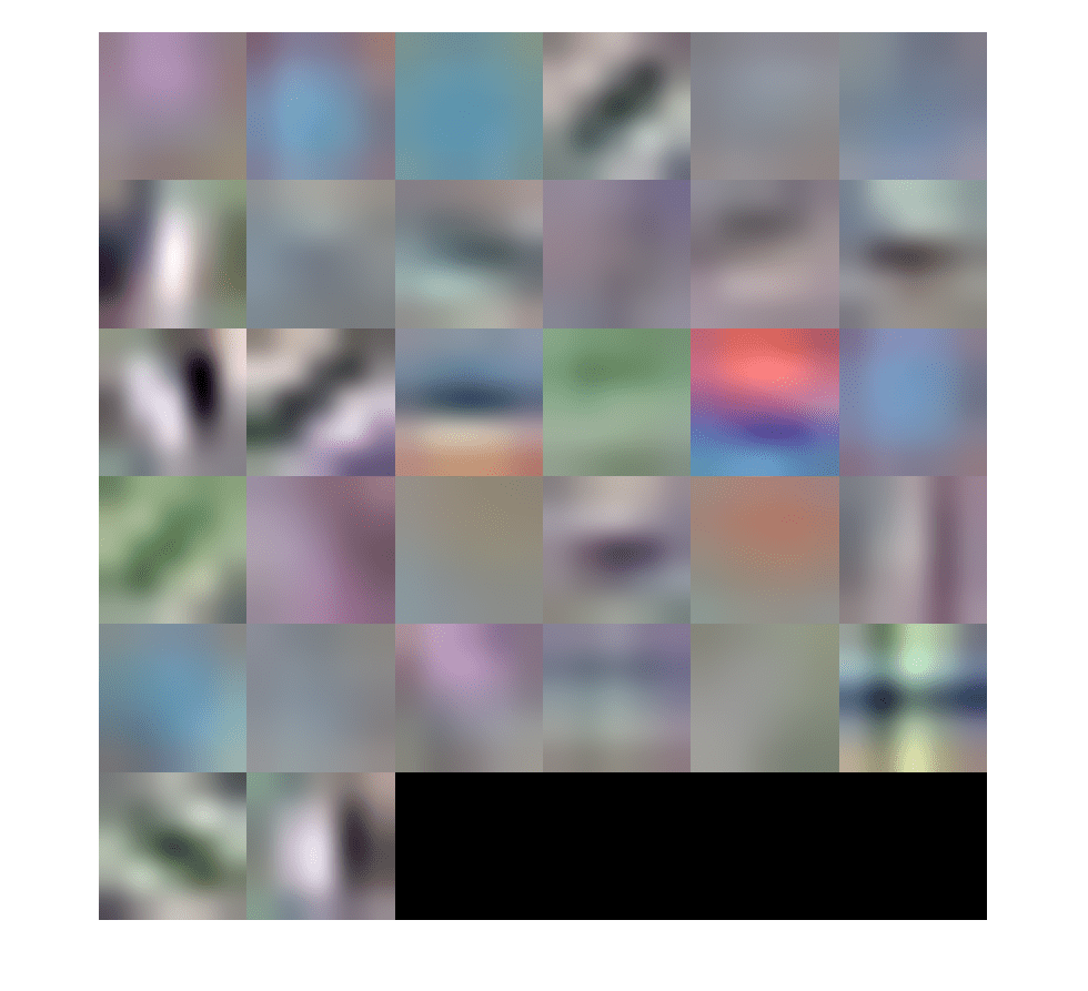
最初の層の重みには、明確な構造がなければなりません。重みがまだランダムな場合は、ネットワークに追加学習が必要であることを示しています。この例の場合、上記のように、最初の層のフィルターが CIFAR-10 学習データからエッジのような特徴を学習しています。

学習の結果を完全に検証するには、CIFAR-10 テストデータを使用してネットワークの分類精度を測定します。精度のスコアが低い場合、追加学習または追加の学習データが必要であることを意味します。この例の目的は、テストセットで 100% の精度を達成することではなく、オブジェクト検出器の学習に使用するのに十分なネットワークの学習を行うことです。

% Run the network on the test set.
YTest = classify(cifar10Net, testImages);

% Calculate the accuracy.
accuracy = sum(YTest == testLabels)/numel(testLabels)

accuracy = 0.7456

追加学習を行うと精度が向上しますが、R-CNN オブジェクト検出器の学習という目的には必要ありません。

学習データの読み込み

ネットワークが CIFAR-10 の分類タスクに対して適切に機能するようになったので、転移学習の手法を使用して、一時停止標識検出のためにネットワークを微調整できます。

最初に、一時停止標識のグラウンドトゥルースデータを読み込みます。

% Load the ground truth data
data = load('stopSignsAndCars.mat', 'stopSignsAndCars');
stopSignsAndCars = data.stopSignsAndCars;

% Update the path to the image files to match the local file system
visiondata = fullfile(toolboxdir('vision'),'visiondata');
stopSignsAndCars.imageFilename = fullfile(visiondata, stopSignsAndCars.imageFilename);

% Display a summary of the ground truth data
summary(stopSignsAndCars)

Variables:
    imageFilename: 41×1 cell array of character vectors
    stopSign: 41×1 cell
    carRear: 41×1 cell
    carFront: 41×1 cell

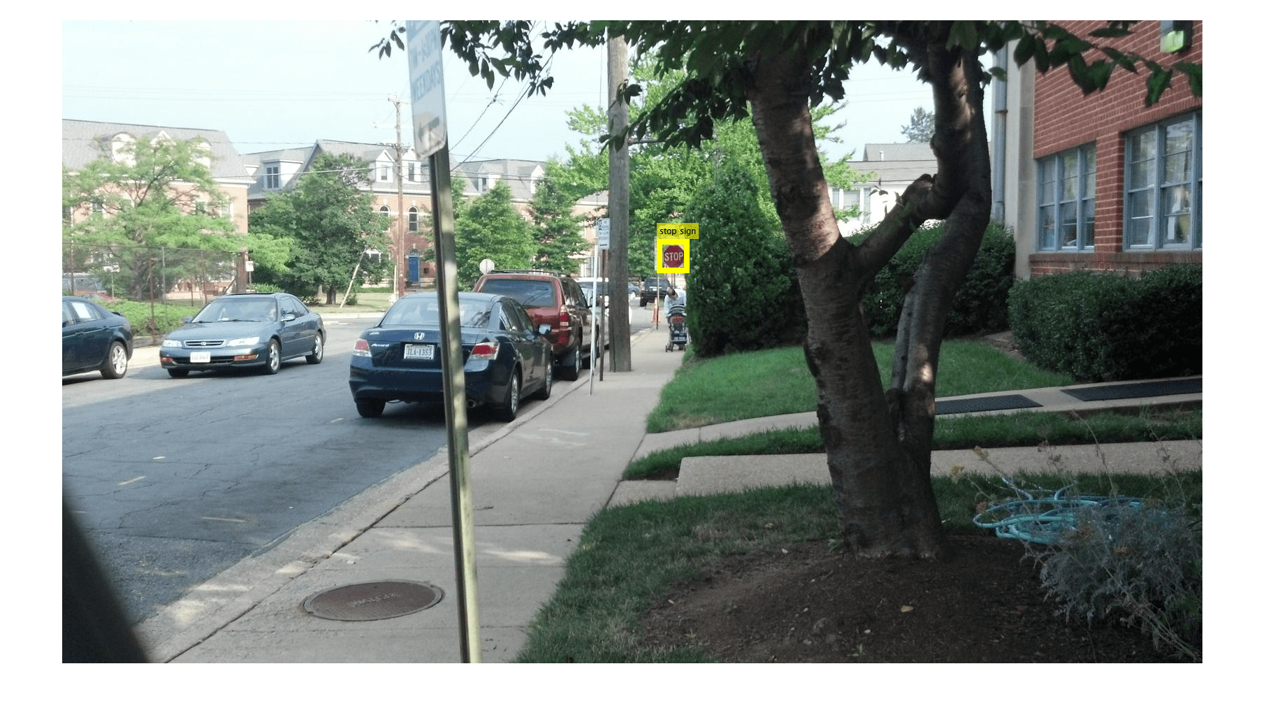
学習データは、一時停止標識、車体前部および後部のイメージファイル名と ROI ラベルが含まれる table 内に格納されています。各 ROI ラベルは、イメージ内で対象オブジェクトの周りの境界ボックスです。一時停止標識検出器の学習には、一時停止標識の ROI ラベルのみが必要です。車体前部および後部の ROI ラベルは削除しなければなりません。

% Only keep the image file names and the stop sign ROI labels
stopSigns = stopSignsAndCars(:, {'imageFilename','stopSign'});

% Display one training image and the ground truth bounding boxes
I = imread(stopSigns.imageFilename{1});
I = insertObjectAnnotation(I,'Rectangle',stopSigns.stopSign{1},'stop sign','LineWidth',8);

figure
imshow(I)

このデータセットには 41 個の学習イメージしかないことに注意してください。41 個のイメージだけを使用して R-CNN オブジェクト検出器の学習をゼロから行うのは実用的でなく、信頼性の高い一時停止標識検出器を生成することはできません。大きなデータセット (CIFAR-10 に含まれる学習イメージは 50,000 個) で事前学習済みのネットワークを微調整して一時停止標識検出器の学習を行うため、はるかに小さいデータセットを使用することが可能になります。

R-CNN 一時停止標識検出器の学習

最後に、trainRCNNObjectDetectorを使用して R-CNN オブジェクト検出器に学習させます。この関数への入力はグラウンドトゥルース table です。この table には、ラベル付きの一時停止標識イメージ、事前学習済みの CIFAR-10 ネットワーク、および学習オプションが含まれています。学習関数は、イメージが 10 個のカテゴリに分類されている元の CIFAR-10 ネットワークを、自動的に 1 つのネットワークに変更します。変更後のネットワークでは、一時停止標識クラスと汎用背景クラスの 2 つのクラスにイメージを分類できます。

学習中、グラウンドトゥルースデータから抽出されたイメージパッチを使用して入力ネットワークの重みが微調整されます。'PositiveOverlapRange' および 'NegativeOverlapRange' パラメーターによって、学習に使用されるイメージパッチが制御されます。学習のポジティブサンプルは、境界ボックスの Intersection over Union メトリクスで測定した場合に、グラウンドトゥルースボックスとのオーバーラップが 0.5 ～ 1.0 のサンプルです。学習のネガティブサンプルは、オーバーラップが 0 ～ 0.3 のサンプルです。これらのパラメーターの最適な値は、学習済みの検出器を検証セットでテストすることによって選択します。

R-CNN の学習の場合、"学習時間を短縮するために MATLAB ワーカーの並列プールの使用が強く推奨されます"。trainRCNNObjectDetector は、Computer Vision Toolbox の基本設定に基づいて並列プールを自動的に作成して使用します。学習の前に並列プールの使用が有効になっていることを確認します。

この例の実行時間を節約するために、事前学習済みのネットワークをディスクから読み込みます。ネットワークを自分で学習させる場合は、以下の変数 doTraining を true に設定します。

学習には、CUDA 対応 NVIDIA™ GPU の使用が強く推奨されます。

% A trained detector is loaded from disk to save time when running the
% example. Set this flag to true to train the detector.
doTraining = false;

if doTraining
    
    % Set training options
    options = trainingOptions('sgdm', ...
        'MiniBatchSize', 128, ...
        'InitialLearnRate', 1e-3, ...
        'LearnRateSchedule', 'piecewise', ...
        'LearnRateDropFactor', 0.1, ...
        'LearnRateDropPeriod', 100, ...
        'MaxEpochs', 100, ...
        'Verbose', true);
    
    % Train an R-CNN object detector. This will take several minutes.    
    rcnn = trainRCNNObjectDetector(stopSigns, cifar10Net, options, ...
    'NegativeOverlapRange', [0 0.3], 'PositiveOverlapRange',[0.5 1])
else
    % Load pre-trained network for the example.
    load('rcnnStopSigns.mat','rcnn')       
end

R-CNN 一時停止標識検出器のテスト

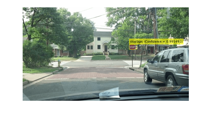
R-CNN オブジェクト検出器を使用してイメージ内の一時停止標識を検出できるようになりました。テストイメージで試してみます。

% Read test image
testImage = imread('stopSignTest.jpg');

% Detect stop signs
[bboxes,score,label] = detect(rcnn,testImage,'MiniBatchSize',128)

bboxes = 1×4

   419   147    31    20

score = single
    0.9955

label = categorical categorical
     stopSign

R-CNN オブジェクトの detect メソッドは、オブジェクトの境界ボックス、検出スコアおよび各検出のクラスラベルを返します。ラベルは、一時停止標識、対向車優先標識、速度制限標識など、複数のオブジェクトを検出する場合に役立ちます。0 ～ 1 で表されるスコアは検出の信頼度を示し、これを使用して低スコアの検出を無視することができます。

% Display the detection results
[score, idx] = max(score);

bbox = bboxes(idx, :);
annotation = sprintf('%s: (Confidence = %f)', label(idx), score);

outputImage = insertObjectAnnotation(testImage, 'rectangle', bbox, annotation);

figure
imshow(outputImage)

デバッグのヒント

R-CNN 検出器内で使用されるネットワークは、テストイメージ全体の処理にも使用できます。ネットワークの入力サイズより大きい、イメージ全体を直接処理することで、分類スコアの 2 次元ヒートマップを生成できます。これは、ネットワークを混乱させているイメージ内の項目を特定して学習を改善する手掛かりを与えてくれる、便利なデバッグツールになります。

% The trained network is stored within the R-CNN detector
rcnn.Network

ans = 
  SeriesNetwork with properties:

    Layers: [15×1 nnet.cnn.layer.Layer]

ネットワークの 14 番目の層であるソフトマックス層から activations (Deep Learning Toolbox) を抽出します。これは、ネットワークがイメージをスキャンするときに生成される分類スコアです。

featureMap = activations(rcnn.Network, testImage, 14);

% The softmax activations are stored in a 3-D array.
size(featureMap)

ans = 1×3

    43    78     2

featureMap の 3 番目の次元はオブジェクトクラスに対応します。

rcnn.ClassNames

ans = 2×1 cell
    {'stopSign'  }
    {'Background'}

一時停止標識の特徴マップは、最初のチャネルに保存されています。

stopSignMap = featureMap(:, :, 1);

アクティベーションの出力のサイズは、ネットワークでのダウンサンプリング演算によって入力イメージより小さくなります。可視性を向上するには、stopSignMap のサイズを入力イメージのサイズに変更します。これはアクティベーションをイメージピクセルにマッピングする非常に大まかな近似であり、図示のみを目的として使用します。

% Resize stopSignMap for visualization
[height, width, ~] = size(testImage);
stopSignMap = imresize(stopSignMap, [height, width]);

% Visualize the feature map superimposed on the test image. 
featureMapOnImage = imfuse(testImage, stopSignMap); 

figure
imshow(featureMapOnImage)

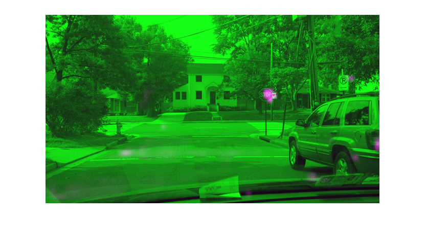
テストイメージ内の一時停止標識は、ネットワークアクティベーションの最大ピークにうまく対応しています。これにより、R-CNN 検出器内で使用されている CNN が実際に一時停止標識を特定できるようになったことを確認できます。他のピークがある場合、誤検知を防ぐため、学習に追加のネガティブデータが必要になることがあります。このような場合には、trainingOptions で 'MaxEpochs' の値を大きくして再学習を行います。

まとめ

この例では、CIFAR-10 データで学習済みのネットワークを使用して R-CNN 一時停止標識オブジェクト検出器に学習させる方法を説明しました。深層学習を使用して他のオブジェクト検出器の学習を行う際にも、同様の手順に従ってください。

参照

[1] Girshick, R., J. Donahue, T. Darrell, and J. Malik. "Rich Feature Hierarchies for Accurate Object Detection and Semantic Segmentation." Proceedings of the 2014 IEEE Conference on Computer Vision and Pattern Recognition. Columbus, OH, June 2014, pp. 580-587.

[2] Deng, J., W. Dong, R. Socher, L.-J. Li, K. Li, and L. Fei-Fei. "ImageNet: A Large-Scale Hierarchical Image Database." Proceedings of the 2009 IEEE Conference on Computer Vision and Pattern Recognition. Miami, FL, June 2009, pp. 248-255.

[3] Krizhevsky, A., and G. Hinton. "Learning multiple layers of features from tiny images." Master's Thesis, University of Toronto. Toronto, Canada, 2009.

[4] https://code.google.com/p/cuda-convnet/

参考