sliceMetrics
Description
sliceMetrics computes group metrics on slices of data using a
trained machine learning model (that is, a binary classifier or a regression model). You can
use the metrics to determine whether the model performs similarly across the slices of
data.
After creating a sliceMetrics object, use the report function to
generate a slice metrics report, or use the plot function to
create a bar graph of a slice metric. Some metrics directly compare data slices to their
complements. The complement of a data slice consists of all observations that are not in the
data slice.
Creation
Syntax
Description
Input Arguments
Properties
Examples
Train a binary classifier on numeric data. Use sliceMetrics to slice the training data according to one of the predictors. Evaluate the accuracy of the model predictions on the data slices.
Load the sample file fisheriris.csv, which contains iris data including sepal length, sepal width, petal width, and species type. Read the file into a table, and then convert the Species variable into a categorical variable. Display the first eight observations in the table.
fisheriris = readtable("fisheriris.csv");
fisheriris.Species = categorical(fisheriris.Species);
head(fisheriris)
SepalLength SepalWidth PetalLength PetalWidth Species
___________ __________ ___________ __________ _______
5.1 3.5 1.4 0.2 setosa
4.9 3 1.4 0.2 setosa
4.7 3.2 1.3 0.2 setosa
4.6 3.1 1.5 0.2 setosa
5 3.6 1.4 0.2 setosa
5.4 3.9 1.7 0.4 setosa
4.6 3.4 1.4 0.3 setosa
5 3.4 1.5 0.2 setosa
Separate the data for two of the iris species: versicolor and virginica.
versicolorData = fisheriris(fisheriris.Species=="versicolor",:);
virginicaData = fisheriris(fisheriris.Species=="virginica",:);
trainingData = [versicolorData;virginicaData];
Train a binary tree classifier on the versicolor and virginica data.
Mdl = fitctree(trainingData,"Species")Mdl =
ClassificationTree
PredictorNames: {'SepalLength' 'SepalWidth' 'PetalLength' 'PetalWidth'}
ResponseName: 'Species'
CategoricalPredictors: []
ClassNames: [versicolor virginica]
ScoreTransform: 'none'
NumObservations: 100
Properties, Methods
Mdl is a ClassificationTree model object trained on 100 observations.
Compute metrics on the training data slices determined by petal length. Because PetalLength is a numeric predictor, sliceMetrics creates data slices by binning the petal length values of observations in Mdl.X. Data slices always partition the data.
sliceResults = sliceMetrics(Mdl,"PetalLength")sliceResults =
sliceMetrics evaluated on PetalLength slices:
PetalLength NumObservations Accuracy OddsRatio PValue EffectSize
___________ _______________ ________ _________ ________ __________
[3, 3.65) 6 1 0 0.083246 -0.031915
[3.65, 4.3) 17 1 0 0.083241 -0.036145
[4.3, 4.95) 31 0.96774 1.1167 0.93193 0.0032726
[4.95, 5.6) 21 0.90476 8.2105 0.23003 0.08258
[5.6, 6.25) 19 1 0 0.08324 -0.037037
[6.25, 6.9] 6 1 0 0.083246 -0.031915
Properties, Methods
In this example, sliceMetrics creates six data slices. The accuracy for each data slice is quite high (over 90%).
Visualize the accuracy for each slice and its complement in Mdl.X.
plot(sliceResults)
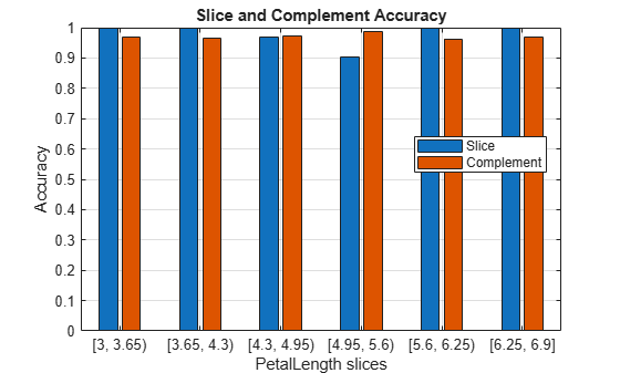
In general, the accuracy for each slice is similar to the accuracy for its slice complement. However, the observations with petal lengths in the range [4.95,5.6) have a slightly lower percentage of correct classifications than all other observations.
Train a regression model using a mix of numeric and categorical data. Use sliceMetrics to compute metrics on a specified data slice of interest.
Load the carbig data set, which contains measurements of cars made in the 1970s and early 1980s. Convert the Origin data to a categorical variable, and combine the variable with a subset of the other measurements into a table.
load carbig
Origin = categorical(cellstr(Origin));
cars = table(Acceleration,Cylinders,Displacement,Horsepower, ...
    Origin,Weight,MPG);
Remove observations with missing values from the cars table. Then, display the first eight observations in the table.
cars = rmmissing(cars);
head(cars)
    Acceleration    Cylinders    Displacement    Horsepower    Origin    Weight    MPG
    ____________    _________    ____________    __________    ______    ______    ___

          12            8            307            130         USA       3504     18
        11.5            8            350            165         USA       3693     15
          11            8            318            150         USA       3436     18
          12            8            304            150         USA       3433     16
        10.5            8            302            140         USA       3449     17
          10            8            429            198         USA       4341     15
           9            8            454            220         USA       4354     14
         8.5            8            440            215         USA       4312     14
Partition the data into training data and test data. Reserve approximately 50% of the observations for computing slice metrics, and use the rest of the observations for model training.
rng(0,"twister") % For reproducibility
cv = cvpartition(length(cars.MPG),Holdout=0.5);
trainingCars = cars(training(cv),:);
testCars = cars(test(cv),:);
Train a Gaussian process regression model using the training data. Standardize the numeric predictors before fitting the model.
Mdl = fitrgp(trainingCars,"MPG",Standardize=true)Mdl =
RegressionGP
PredictorNames: {'Acceleration' 'Cylinders' 'Displacement' 'Horsepower' 'Origin' 'Weight'}
ResponseName: 'MPG'
CategoricalPredictors: 5
ResponseTransform: 'none'
NumObservations: 196
KernelFunction: 'SquaredExponential'
KernelInformation: [1×1 struct]
BasisFunction: 'Constant'
Beta: 25.8166
Sigma: 3.9677
PredictorLocation: [11×1 double]
PredictorScale: [11×1 double]
Alpha: [196×1 double]
ActiveSetVectors: [196×11 double]
PredictMethod: 'Exact'
ActiveSetSize: 196
FitMethod: 'Exact'
ActiveSetMethod: 'Random'
IsActiveSetVector: [196×1 logical]
LogLikelihood: -566.1334
ActiveSetHistory: []
BCDInformation: []
Properties, Methods
Mdl is a RegressionGP model object trained on a mix of numeric and categorical predictors.
Create a data slice of the test set cars manufactured in the USA with an acceleration value of 15 or more.
testDataSliceIndex = testCars.Origin=="USA" & testCars.Acceleration >= 15;Evaluate the regression model on the custom data slice using the sliceMetrics function. Use the report function to display the mean squared error (MSE), a two-sample t-statistic, and a two-sample p-value for the custom data slice (true) and its complement (false).
sliceResults = sliceMetrics(Mdl,testCars,testDataSliceIndex);
metricsTbl = report(sliceResults,Metrics=["mse","tstat","pvalue"])
metricsTbl=2×5 table
    custom    NumObservations    Error     TStatistic     PValue
    ______    _______________    ______    __________    ________

    true             61           9.624     -1.8661      0.063547
    false           135          16.036      1.8661      0.063547
The MSE is smaller for the custom data slice than for the remaining test set observations. However, the t-statistic and p-value for Welch's t-test indicate that the mean of the squared errors is not statistically different at the 5% significance level between the slice and its complement.
Train a regression model on a mix of numeric and categorical data. Use sliceMetrics to slice the test data according to two predictors. Compute the mean squared error for the data slices. To improve the general model performance across the data slices, generate synthetic observations and use them to retrain the model.
Load the carbig data set, which contains measurements of cars made in the 1970s and early 1980s. Bin the Model_Year data to form a categorical variable, and combine the variable with a subset of the other measurements into a table. Remove observations with missing values from the table. Then, display the first eight observations in the table.
load carbig
ModelDecade = discretize(Model_Year,[70 80 89], ...
    "categorical",["70s","80s"]);
ModelDecade = categorical(ModelDecade,Ordinal=false);
cars = table(Acceleration,Displacement,Horsepower, ...
    ModelDecade,Weight,MPG);
cars = rmmissing(cars);
head(cars)
    Acceleration    Displacement    Horsepower    ModelDecade    Weight    MPG
    ____________    ____________    __________    ___________    ______    ___

          12            307            130            70s         3504     18
        11.5            350            165            70s         3693     15
          11            318            150            70s         3436     18
          12            304            150            70s         3433     16
        10.5            302            140            70s         3449     17
          10            429            198            70s         4341     15
           9            454            220            70s         4354     14
         8.5            440            215            70s         4312     14
Partition the data into training data and test data. Reserve approximately 50% of the observations for computing slice metrics, and use the rest of the observations for model training.
rng(0,"twister") % For reproducibility of partition
cv = cvpartition(length(cars.MPG),Holdout=0.5);
trainingCars = cars(training(cv),:);
testCars = cars(test(cv),:);
Train a regression tree model using the training data. Then, compute metrics on the test data slices determined by the decade of manufacture and the weight of the car. Partition the numeric Weight values into three bins. Because ModelDecade is a categorical variable with two categories, sliceMetrics creates six data slices.
Mdl = fitrtree(trainingCars,"MPG");
sliceResults = sliceMetrics(Mdl,testCars,["ModelDecade","Weight"], ...
    NumBins=3)
sliceResults =
sliceMetrics evaluated on ModelDecade and Weight slices:

    ModelDecade         Weight         NumObservations    Error     TStatistic      PValue      EffectSize
    ___________    ________________    _______________    ______    __________    __________    __________

        70s        [1649, 2812.7)            64           18.392     0.23812         0.81224      1.3097
        70s        [2812.7, 3976.3)          53           6.6804     -4.3456      2.3745e-05     -14.843
        70s        [3976.3, 5140]            36           5.6089     -4.7484      4.0884e-06     -14.578
        80s        [1649, 2812.7)            32           30.874      2.2891         0.02727      15.972
        80s        [2812.7, 3976.3)          11           64.626      2.4672        0.032784      49.918
        80s        [3976.3, 5140]             0              NaN         NaN             NaN         NaN


  Properties, Methods
For the cars made in the 80s with a weight in the range [2812.7,3976.3) (that is, the observations in slice 5), the mean squared error (MSE) is much higher than the MSE for the cars in the other data slices.
Generate 500 synthetic observations using the synthesizeTabularData function. By default, the function uses a binning technique to learn the distribution of the variables in trainingCars before synthesizing the data.
rng(10,"twister") % For reproducibility of data generation
syntheticCars = synthesizeTabularData(trainingCars,500);
Combine the training observations with the synthetic observations. Use the combined data to retrain the regression tree model.
newTrainingCars = [trainingCars;syntheticCars];
newMdl = fitrtree(newTrainingCars,"MPG");
Compute metrics on the same test data slices using the retrained model.
newSliceResults = sliceMetrics(newMdl,testCars,["ModelDecade","Weight"], ...
    NumBins=3)
newSliceResults =
sliceMetrics evaluated on ModelDecade and Weight slices:

    ModelDecade         Weight         NumObservations    Error     TStatistic      PValue      EffectSize
    ___________    ________________    _______________    ______    __________    __________    __________

        70s        [1649, 2812.7)            64           20.986      1.5012         0.13736      8.5476
        70s        [2812.7, 3976.3)          53           9.9331     -2.0166        0.045209     -7.2595
        70s        [3976.3, 5140]            36           5.4484     -4.3062      2.6575e-05     -11.982
        80s        [1649, 2812.7)            32           20.422      1.0664         0.29206       6.206
        80s        [2812.7, 3976.3)          11           24.162      1.0643         0.30927       9.463
        80s        [3976.3, 5140]             0              NaN         NaN             NaN         NaN


  Properties, Methods
Visually compare the MSE values for the data slices.
tiledlayout(1,2)

nexttile
plot(sliceResults)
ylim([0 70])
xticklabels(1:6)
legend(Location="northwest")

nexttile
plot(newSliceResults)
ylim([0 70])
xticklabels(1:6)
legend(Location="northwest")
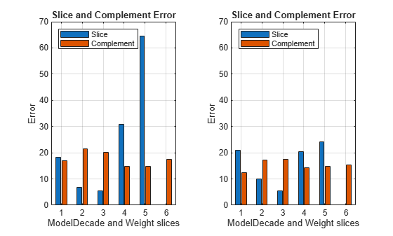
The MSE for slice 5 is lower for the model trained with the training and synthetic observations (newMdl) than for the model trained with only the training data (Mdl).
Tips
If your model does not perform well across all data slices, you can try the following:
Retrain your model using different observation weights.
Collect new data or generate synthetic data before retraining your model. For an example, see Improve Performance on Data Slices Using Synthetic Data.
Algorithms
References
[1] Chung, Yeounoh, Tim Kraska, Neoklis Polyzotis, Ki Hyun Tae, and Steven Euijong Whang. “Automated Data Slicing for Model Validation: A Big Data - AI Integration Approach.” IEEE Transactions on Knowledge and Data Engineering 32, no. 12 (2020): 2284–96.
Version History
Introduced in R2026a