Identification of NARMAX Models

This example describes some ways of identifying nonlinear auto-regressive models with moving average terms, commonly known as NARMAX models. Such models are currently not available in System Identification Toolbox™. However, as this example shows, they can be easily generated using the available model structures and their training algorithms. The main extra work involved is in the preparation of a finite-horizon prediction algorithm.

Introduction

Nonlinear Auto-Regressive with Exogenous Inputs (NARMAX) are nonlinear counterparts of the linear auto-regressive models that are popular structures employed for forecasting the future outcomes of time series. In order to understand the structure of a NARMAX model, it is useful to review its simpler versions first.

Linear Auto-Regressive Models

In its simplest form, a linear auto-regressive model (AR) takes the form:

$$y(k)+a_{1}y(k-1)+a_{2}y(k-2)+\dots =e(k)$$

or

$$A(q)y(k)=e(k)$$, where $$A(q)=1+a_1{q}^{-1}+a_2{q}^{-2}+\dots$$ is an polynomial in the shift operator $$q^{-1}$$ (that is, $$q^{-i}y(k)=y(k-i)$$).

$$y(k)$$ describes the time series under observation and e(k) is the disturbance process. Thus $$y(k)$$ is generated by a weighted sum of its own past values but corrupted by the noise $$e(k)$$. Let us call this the data-generating system (sometimes also called the true system), In engineering applications, $$y(k)$$ is typically obtained by sampling a signal of physical origin, $$y(t)$$, such as vibrations measured using an accelerometer. When $$y(t)$$ is sampled uniformly using a sampling interval (also called sample time) of $$T_s$$, this leads to the measurements $$y(T_s),y(2T_s),\dots ,y(N{T}_s)$$, where $$k=1,\dots N$$ are the sampling instants. Typically, $$e(t)$$ is assumed to be a zero mean i.i.d. gaussian process. Then given the measurements $$y(k),k=1,2,\dots ,T$$, the prediction of the response at the next time instant $$T+1$$ is given by:

$$\underset{}{\overset{\sim }{y}}(T+1)=-a_{1}y(T)-a_2(T-1)+\dots$$

This equation is called the one-step-ahead predictor for the process $$y(k)$$. Its purpose is to predict what the value of $$y$$ will be exactly one step into the future. When exogenous but measurable influences $$u(k)$$ affect $$y(k)$$, the data-generating equation takes the form:

$\mathit{y}\left(\mathit{k}\right)+{\mathit{a}}_1\mathit{y}\left(\mathit{k}-1\right)+{\mathit{a}}_2\mathit{y}\left(\mathit{k}-2\right)+\dots ={\mathit{b}}_0\mathit{u}\left(\mathit{k}\right)+{\mathit{b}}_1\mathit{u}\left(\mathit{k}-1\right)+\dots +\mathit{e}\left(\mathit{k}\right)$, or more succinctly:

$$\mathit{A}\left(\mathit{q}\right)\mathit{y}\left(\mathit{k}\right)=\mathit{B}\left(\mathit{q}\right)\mathit{u}\left(\mathit{k}\right)+\mathit{e}\left(\mathit{k}\right)$$

where $$A(q):=1+a_1{q}^{-1}+a_2{q}^{-2}+\dots$$and $$B(q):=b_0+b_1{q}^{-1}+\dots$$

This is called an Auto-Regressive with Exogenous Input (ARX) model. Some observations regarding the ARX model structure:

• $$u(k)$$ is supposed to be known or measured with no noise (practically, any measurement errors in $$u(k)$$ are combined into the fictitious noise source $$e(k)$$).

• The model regressors are the lagged variables $$y(k-1),y(k-2),\dots ,u(k),u(k-1),u(k-2),\dots .$$ Note that at time instant $$k$$, the regressors are fully known.

• In engineering applications, $$y(t)$$ is referred to as an output signal, and $$u(t)$$ an input signal. Thus the data-generating equation can be viewed as an input-output model.

The one-step-ahead predictor takes the form:

$$\underset{}{\overset{\sim }{y}}(k+1)=-a_{1}y(k)-a_{2}y(k-1)+\dots ,b_{0}u(k+1)+b_{1}u(k)+b_{2}u(k-1)+\dots$$

An ARX model can also be expressed in the state-space form by defining the states using the lagged variables. The predictor of the AR or the ARX model is a static equation - the terms on the right hard side of the predictor equations are fully known at the time instant $$k$$ and do not need to look up their past values. However, things get complicated when the output in the data-generating system is affected by not just the current value of the disturbance $$e(k)$$ but also its past values ($$e(k-1),e(k-2)$$, etc). For example, an Auto-Regressive with Moving Average (ARMA) model takes the form:

$$y(k)=a_{1}y(k-1)+a_{2}y(k-2)+\dots +e(k)+c_{1}e(k-1)+c_{2}e(k-2)+\dots$$

Here, the one-step-ahead prediction of $$y(k)$$ is not as straightforward as before; one needs to be know the past predictions ($$\underset{}{\overset{\sim }{y}}(k),\underset{}{\overset{\sim }{y}}(k-1),\dots$$) in order to estimate $$\underset{}{\overset{\sim }{y}}(k+1)$$. When exogenous inputs are present, the ARMA model becomes an ARMAX model with the suffix "X" denoting the presence of exogenous inputs.

$$y(k)=a_{1}y(k-1)+a_{2}y(k-2)+\dots +b_{0}u(k)+b_{1}u(k-1)+\dots +e(k)+c_{1}e(k-1)+c_{2}e(k-2)+\dots$$

An ARMA predictor is:

$$\underset{}{\overset{\sim }{y}}(k)=a_{1}y(k-1)+a_{2}y(k-2)+\dots +c_1(y(k-1)-\underset{}{\overset{\sim }{y}}(k-1))+c_2(y(k-2)-\underset{}{\overset{\sim }{y}}(k-2))+\dots$$

Rearranging:

$$\underset{}{\overset{\sim }{y}}(k)+c_1\underset{}{\overset{\sim }{y}}(k-1)+\underset{}{\overset{\sim }{y}}(k-2)+\dots =(a_1+c_1)y(k-1)+(a_2+c_2)y(k-2)+\dots$$

This is an auto-regressive equation. We do not know the value of $$\underset{}{\overset{\sim }{y}}(k)$$ in advance. Only the initial value/guess for $$\underset{}{\overset{\sim }{y}}(1)$$ is available. This model must be simulated - use the initial guess $$\underset{}{\overset{\sim }{y}}(1)$$ to solve for $$\underset{}{\overset{\sim }{y}}(2)$$, and then use $$\underset{}{\overset{\sim }{y}}(1),\underset{}{\overset{\sim }{y}}(2)$$ values to solve for $$\underset{}{\overset{\sim }{y}}(3)$$, etc.

Nonlinear Auto-Regressive Models

Referring to the predictor for the ARX model, notice two facts:

1. The regressors are all lagged versions of the measured variables $$y(k)$$ and $$u(k)$$ with no other transformations.

2. The prediction uses a weighted sum of the regressors.

An nonlinear extension of the linear ARX predictor can be realized as follows:

1. In place of linear regressors ($$y(k-1),y(k-2),\dots ,u(k-1),\dots$$), one can use nonlinear transformations such as polynomials or trigonometric transformations of the lagged variables, for example, $$y(k-1{)}^2,y(k-4)u(k-6),sin(3u(t-5)),|u(t){|}^3,\dots$$

2. The simple weighted sum can be replaced by a more complicated nonlinear map such as sigmoids or wavelets.

Such extensions are facilitated by the Nonlinear ARX (NARX) models. These models take the generic form:

$$\mathit{y}\left(\mathit{k}\right)=\mathit{f}\left({\mathit{r}}_1\left(\mathit{k}\right),{\mathit{r}}_2\left(\mathit{k}\right),\dots ,\right)+\mathit{e}\left(\mathit{k}\right)$$

where ${\mathit{r}}_1\left(\mathit{k}\right),{\mathit{r}}_2\left(\mathit{k}\right),\dots$are the model regressors. For example, ${\mathit{r}}_1\left(\mathit{k}\right)=\mathit{y}\left(\mathit{k}-1\right),{\mathit{r}}_2\left(\mathit{k}\right)={\mathit{y}\left(\mathit{k}-5\right)}^2,{\mathit{r}}_3\left(\mathit{k}\right)=\sin \left(2\pi \mathit{u}\left(\mathit{k}\right)\right)$, etc. A simpler notation for the NARX models is:

$$\mathit{y}\left(\mathit{k}\right)=\mathit{f}\left(\mathit{y}\left(\mathit{k}-1\right),\mathit{y}\left(\mathit{k}-2\right),\dots ,\mathit{u}\left(\mathit{k}\right),\mathit{u}\left(\mathit{k}-1\right),\dots \right)+\mathit{e}\left(\mathit{k}\right)$$

where it is understood that the lagged variables may undergo additional transformations (polynomial, trigonometric etc) before passed as input arguments of the mapping function $$f(\cdot )$$.

The NARX models are represented by the IDNLARX objects. They are trained using the NLARX command.

NARMAX Models

Similar to the linear case, the NARX model can be extended to allow for dependence on the past prediction errors leading to the NARMAX model form:

$$\mathit{y}\left(\mathit{k}\right)=\mathit{f}\left(\mathit{y}\left(\mathit{k}-1\right),\mathit{y}\left(\mathit{k}-2\right),\dots ,\mathit{u}\left(\mathit{k}\right),\mathit{u}\left(\mathit{k}-1\right),\dots \mathit{e}\left(\mathit{k}-1\right),\mathit{e}\left(\mathit{k}-2\right),\dots \right)+\mathit{e}\left(\mathit{k}\right)$$

In this form, $$e(k-1),e(k-2),\dots$$can be viewed as extra regressors whose values are not known directly. Note that at time $$k$$, $$e(k-i)=y(t-i)-\underset{}{\overset{\sim }{y}}(t-i)$$, so the one-step-ahead predictor takes the form:

$$\stackrel{\sim }{\mathit{y}}\left(\mathit{k}+1\right)=\mathit{f}\left(\mathit{y}\left(\mathit{k}\right),\mathit{y}\left(\mathit{k}-1\right),\dots ,\mathit{u}\left(\mathit{k}+1\right),\mathit{u}\left(\mathit{k}\right),\mathit{u}\left(\mathit{k}-1\right),\dots \stackrel{\sim }{\mathit{y}}\left(\mathit{k}\right),\stackrel{\sim }{\mathit{y}}\left(\mathit{k}-1\right),\stackrel{\sim }{\mathit{y}}\left(\mathit{k}-2\right),\dots \right)$$

Since the predictions depend upon their own past values, determining $\stackrel{\sim }{\mathit{y}}\left(\mathit{k}+1\right)$ requires simulation - starting at $\stackrel{\sim }{\mathit{y}}\left(1\right)$ and marching forward to the current time instant $$k$$. This makes the prediction more time-consuming. Also the recursive nature of the prediction implies that the model training to determine $$f(\cdot )$$ is more complex.

Some examples of creating NARMAX models are described in the next sections.

Example Setup

Consider a scalar time-series "y", that is observed for 1000 seconds at an interval of 1 second. The values of y are influenced by an exogenous input "u". The observations of u and y are recorded in a timetable TT. In the standard system identification terminology, TT represents the observations of a single-input, single-output system.

load NARMAXExampleData TT
stackedplot(TT)

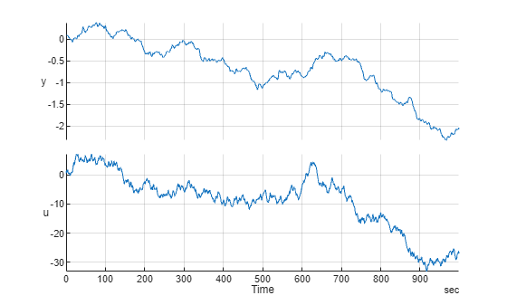
grid on

Use the first half of the data for all model training exercises while reserving the second half for validation of the results.

% Prepare training and validation data
TrainData = TT(1:500,:); 
TrainData.Properties.Description = "Training Data";
ValidateData = TT(501:end,:);
ValidateData.Properties.Description = "Validation Data";
wrn = warning('off','Ident:estimation:NparGTNsamp');
cl = onCleanup(@()warning(wrn));

Linear ARMAX

First, fit a linear ARMAX model to the data for setting a reference. Calling ssest(TT, 1:10) suggests a model order of 2. Using this knowledge, we pick na=nb=nc=2, and nk=1 for the linear ARMAX model; nk=1 means we assume that there is no feedthrough.

na = 2;
nb = 2;
nc = 2;
nk = 1;
sysARMAX = armax(TrainData,[na nb nc nk],InputName="u")

sysARMAX =
Discrete-time ARMAX model: A(z)y(t) = B(z)u(t) + C(z)e(t)
  A(z) = 1 - 0.4184 z^-1 - 0.5859 z^-2                   
                                                         
  B(z) = 0.001209 z^-1 - 0.0009946 z^-2                  
                                                         
  C(z) = 1 + 1.908 z^-1 + 0.9852 z^-2                    
                                                         
Sample time: 1 seconds
  
Parameterization:
   Polynomial orders:   na=2   nb=2   nc=2   nk=1
   Number of free coefficients: 6
   Use "polydata", "getpvec", "getcov" for parameters and their uncertainties.

Status:                                               
Estimated using ARMAX on time domain data "TrainData".
Fit to estimation data: 97.23% (prediction focus)     
FPE: 0.0001116, MSE: 0.0001081                        
 
Model Properties

Check the model performance by its ability to forecast 25 steps into the future.

% Check the model performance on training data
compare(TrainData, sysARMAX, 25)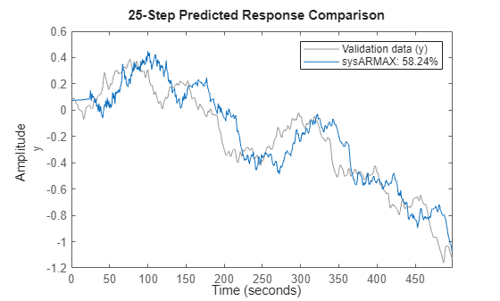 

% Check the model performance on validation data
clf
compare(ValidateData, sysARMAX, 25)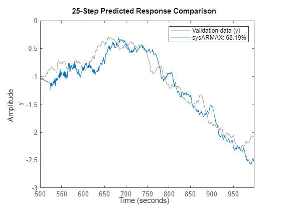 

NARMAX Models with Linear and Additive Moving Average Term

Consider the data-generating system:

$$\mathit{y}\left(\mathit{k}\right)=\mathit{f}\left(\mathit{y}\left(\mathit{k}-1\right),\mathit{y}\left(\mathit{k}-2\right),\dots ,\mathit{u}\left(\mathit{k}\right),\mathit{u}\left(\mathit{k}-1\right),\dots \right)+\mathit{C}\left(\mathit{q}\right)\mathit{e}\left(\mathit{k}\right)$$

Here, the contribution of the error terms has been separated out into a separate additive term $$C(q)e(k)=e(k)+c_{1}e(k-1)+c_{2}e(k-2)+\dots$$The one-step-ahead predictor is:

$$\underset{}{\overset{\sim }{y}}(k+1)=f(y(k),y(k-1),\dots ,u(k+1),u(k),u(k-1),\dots )+c_1(y(k)-\underset{}{\overset{\sim }{y}}(k))+c_2(y(k-1)-\underset{}{\overset{\sim }{y}}(k-1))+\dots$$

Rearranging the predicted quantities, we get:

$$C(q)\underset{}{\overset{\sim }{y}}(k+1)=f(y(k),y(k-1),\dots ,u(k+1),u(k),u(k-1),\dots )+c_{1}y(k)+c_{2}y(k-1)+\dots$$

where $$C(q)=1+c_1{q}^{-1}+c_2{q}^{-2}+\dots$$.This is an auto-regressive model for the process $$\underset{}{\overset{\sim }{y}}(k+1)$$ driven by the inputs $$y(k),u(k)$$ which are assumed to be known at time instant $$k$$. For training this model using input/output measurements $$\{u(k),y(k)\},k=1,2,\dots ,N$$, we need to determine the values of the coefficients (such as weights and biases) used by the nonlinear function $$f(\cdot )$$, as well as the coefficients $$c_1,c_2,\dots$$employed by the moving average terms.

System Identification Toolbox supports estimation of NARX models but not the NARMAX models. However, as this example shows, it is possible to NLARX command together with a grey-box (NLGREYEST) based refinement step to obtain a NARMAX model.

Nonlinear ARX

As a starting step towards building a nonlinear ARMAX model, first, create a NARX model (no MA term) to this data. For this we need two pieces of information - the model regressors and the nature of the function that maps the regressors to the predicted response. We make the following choices:

1. The model uses linear regressors: $$y(k-1),y(k-2),u(k-1),u(k-2),u(k-3)$$. This is consistent with the model orders used for the linear model sysARMAX.

2. Use 2 hidden layers with 5 sigmoid activations each for the nonlinear function that maps the regressors to the output.

The parameters of this model are the various weights and biases used by the fully connected layers of the nonlinear (neural network) function.

% Create regressor functions
Reg = linearRegressor(["y","u"],{1:2, 1:3});  
getreg(Reg)

ans = 5×1 string
    "y(t-1)"
    "y(t-2)"
    "u(t-1)"
    "u(t-2)"
    "u(t-3)"

% Create nonlinear map which is a 2-layer neural network with sigmoid activations
NL = idNeuralNetwork([5 5],"sigmoid", NetworkType="RegressionNeuralNetwork")

NL = 
Multi-Layer Neural Network

 Nonlinear Function: Uninitialized regression neural network
         Contains 2 hidden layers using "sigmoid" activations.
         (uses Statistics and Machine Learning Toolbox)
 Linear Function: uninitialized
 Output Offset: uninitialized

              Network: 'Regression neural network parameters'
            LinearFcn: 'Linear function parameters'
               Offset: 'Offset parameters'
    EstimationOptions: [1×1 struct]

Create a Nonlinear ARX model by training it in closed-loop, that is, by minimizing the simulation errors.

% Prepare estimation options
opt = nlarxOptions(Focus="simulation", Display="on",Normalize=false);
opt.SearchOptions.MaxIterations = 50;

% Train the model
sysNARX = nlarx(TrainData, Reg, NL, opt, OutputName="y")

sysNARX =

Nonlinear ARX model with 1 output and 1 input
  Inputs: u
  Outputs: y

Regressors:
  Linear regressors in variables y, u
  List of all regressors

Output function: Regression neural network
Sample time: 1 seconds

Status:                                               
Estimated using NLARX on time domain data "TrainData".
Fit to estimation data: 70.67% (simulation focus)     
FPE: 0.0006333, MSE: 0.01208                          

Model Properties

sysNARX provides an initial guess of the model coefficients. How well does this model perform? Compute 25 step ahead forecasts.

% Compare 25-step ahead prediction response of the model to 
% the measured output in the training dataset
compare(TrainData, sysNARX, 25) % comparison against the training dataset 

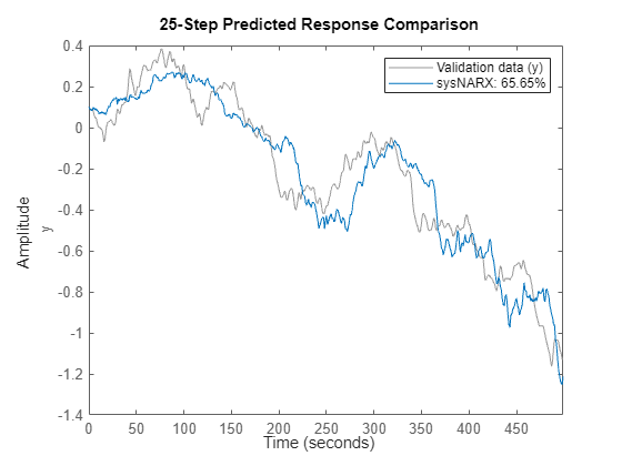
compare(ValidateData, sysNARX, 25) % comparison against the validation dataset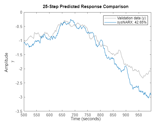

Moving Average Model of the Residuals

Next, compute the prediction errors for the model sysNARX.

errData = pe(TrainData, sysNARX, 1);
stackedplot(errData)

Fit a linear moving-average model to the signal in timetable errData. Assume a $$2^{nd}$$ order process.

nc = 2;
errMA = armax(errData, [0 nc])

errMA =
Discrete-time MA model: y(t) = C(z)e(t)
  C(z) = 1 + 0.6441 z^-1 + 0.1977 z^-2 
                                       
Sample time: 1 seconds
  
Parameterization:
   Polynomial orders:   nc=2
   Number of free coefficients: 2
   Use "polydata", "getpvec", "getcov" for parameters and their uncertainties.

Status:                                             
Estimated using ARMAX on time domain data "errData".
Fit to estimation data: 16.04% (prediction focus)   
FPE: 0.0003317, MSE: 0.0003291                      
 
Model Properties

resid(errData, errMA)

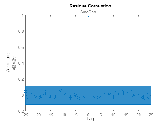
The residual plot shows that the model errMA captures the essential dynamics embedded in the data (errData) since the residuals of this model are mostly uncorrelated at non-zero lags (the blue patch marks the region of statistical insignificance). At this point, an initial guess of the moving average term is:

errMA.C  % C(q) value for the NARMAX model

ans = 1×3

    1.0000    0.6441    0.1977

Grey-Box Refinement of Model Parameters

Our NARMAX model is a combination of the NARX model with a linear moving average term. We refine the initial estimates (as provided by sysNARX and errMA) using a grey-box modeling approach. The parameters of sysNARX are kept fixed in this example in order to speed up the refinement.

% ODE file
type('NARMAX_ODE.m')

%------------------------------------------------------------------
function [dx, y] = NARMAX_ODE(~,x,u,fcn_par,C,varargin) 
%NARMAX_ODE ODE function for refining the coefficients of a NARMAX model 
% using a grey-box approach.
%
% Ther NARMAX model uses an additive moving average term.

% Copyright 2024 The MathWorks, Inc.

% If there are 2 moving average terms, the states are: 
% x1 := y(t-1)
% x2 := y(t-2)
% x3 := y_measured(t-1)
% x4 := y_measured(t-2)
% x5 := u(t-1)
% x6 := u(t-2)
% x7 := u(t-3)

% fcn_par -> coefficients used in f(.)
% C -> free coefficients of the moving average polynomial C(q)
% sys -> Nonlinear ARX model representing the function f(.)

% Separate out the parameters of the nonlinear sigmoidal function 
% and those corresponding to the moving average term
sys = varargin{1}{1};
nc = varargin{1}{2};
% sys = setpvec(sys, fcn_par); % not needed if fcn_par is fixed in the example
NL = sys.OutputFcn;
regressor_vector = x([nc+(1:2), end-2:end])';
y_NL = evaluate(NL,regressor_vector);
y_MA = C'*(x(nc+(1:nc))-x(1:nc));
y = y_NL + y_MA;
 
dx1 = y;
for k=1:nc-1
   dx1 = [dx1; x(k)]; %#ok<*AGROW>
end
dx1(end+1) = u(1);
for k=nc+(1:nc-1)
   dx1 = [dx1; x(k)];
end
dx2 = [u(2); x(end-2); x(end-1)];
dx = [dx1;dx2];

end
%------------------------------------------------------------------

% Prepare the grey-box model
par1 = getpvec(sysNARX);
par2 = errMA.C(2:end)';
par = {par1,par2};
Orders = [1 2 7];
sysGrey_ini = idnlgrey("NARMAX_ODE",Orders,par,zeros(Orders(3),1),1,FileArgument={sysNARX, nc});
sysGrey_ini.Parameters(1).Fixed = 1; % (only update the MA coefficients)
% Training options
greyOpt = nlgreyestOptions(Display="on", SearchMethod="lsq");
Data_grey = iddata(TrainData.y,[TrainData.y, TrainData.u],1,OutputName="y",InputName=["y","u"]);
% Train the model
sysGrey = nlgreyest(Data_grey, sysGrey_ini, greyOpt)

sysGrey =

Discrete-time nonlinear grey-box model defined by 'NARMAX_ODE' (MATLAB file):

   x(t+Ts) = F(t, x(t), u(t), p1, p2, FileArgument)
      y(t) = H(t, x(t), u(t), p1, p2, FileArgument) + e(t)

 with 2 input(s), 7 state(s), 1 output(s), and 2 free parameter(s) (out of 74).

Sample time: 1 seconds

Status:                                                                                      
Estimated using Solver: FixedStepDiscrete; Search: lsqnonlin on time domain data "Data_grey".
Fit to estimation data: 94.96%                                                               
FPE: 0.0003595, MSE: 0.0003566                                                               

Model Properties

sysGrey is a one-step-ahead predictor of $$y(k)$$. Can we use this model for multi-step ahead prediction? The answer is YES. Towards this goal, we first observe the following facts:

1. An N-step ahead prediction can be viewed as a sequence of N one-step-ahead predictions.

2. In many engineering applications, a good model is one that can be used for simulation. Simulation amounts to an infinite-step ahead prediction.

The function predictNARMAX (attached to this example) performs multi-step ahead predictions, including pure simulations.

Next we use the trained model sysGrey to forecast the values of $$y(k)$$. Note that computing just one-step-ahead prediction requires a simulation of the trained model. For the following example, set the prediction horizon to 25 samples, that is, predict the value of $$y(k+25)$$ given data $$y(i),u(i),i=1,\dots ,k$$. To save time, we compute the forecasts for every $$10^{th}$$ sample (see the variable called SKIP in predictNARMAX).

H = 25;
plotPredictions(H, TrainData, sysARMAX, sysNARX, sysGrey);

Prediction started ...done.

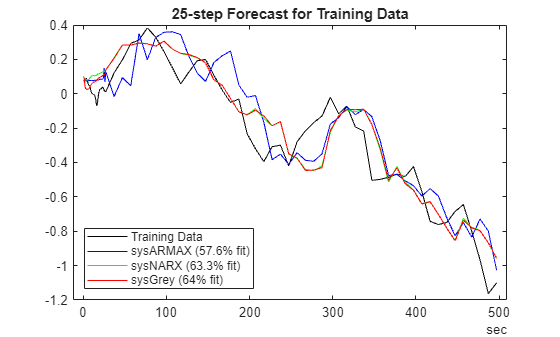
We can similarly generate the forecasting results for the validation dataset.

plotPredictions(H, ValidateData, sysARMAX, sysNARX, sysGrey);

Prediction started ...done.

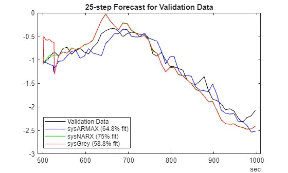
Generic NARMAX Models

In general, we may not know the nature of the dependence of the output $$y(k)$$ on the error terms $$e(k-1),e(k-2),\dots$$Using $$e(k)=y(k)-\underset{}{\overset{\sim }{y}}(k)$$, a generic form of the NARMX predictor is:

$$\stackrel{\sim }{\mathit{y}}\left(\mathit{k}\right)=\mathit{f}\left(\stackrel{\sim }{\mathit{y}}\left(\mathit{k}-1\right),\stackrel{\sim }{\mathit{y}}\left(\mathit{k}-2\right),\dots ,\mathit{y}\left(\mathit{k}-1\right),\mathit{y}\left(\mathit{k}-2\right),\dots ,\mathit{u}\left(\mathit{k}\right),\mathit{u}\left(\mathit{k}-1\right),\dots \right)$$

This is a model that uses the measured processes$\mathit{y}\left(\mathit{k}\right)$ and $\mathit{u}\left(\mathit{k}\right)$ as inputs and generates $\stackrel{\sim }{\mathit{y}}\left(\mathit{k}\right)$as the response. Hence we can approach the determination of the function $$f(\cdot )$$ as a exercise in function approximation using a black-box model. Neural networks can be employed as generic forms of the function. This can be achieved using either the Nonlinear ARX modeling framework, or using the Neural State-Space models.

Using Nonlinear ARX Models

While Nonlinear ARX models are meant for auto-regressive processes with no moving average terms (that is, NARX rather than NARMAX), using the measured output $$y(k)$$ explicitly as an input allows us to use this machinery for identifying NARMAX models, as long as the training takes place in closed-loop (recurrent configuration). This is achieved by setting the estimation focus to "simulation" during model training.

We have two options - train model for 1-steap-ahead prediction or for infinite-horizon. We try both next. First identify a 1-step-ahead predictor model.

One step ahead predictor

% Create regressors
Reg = linearRegressor(["yp","y","u"],{1:2, 1:2, 1:3});  
getreg(Reg)

ans = 7×1 string
    "yp(t-1)"
    "yp(t-2)"
    "y(t-1)"
    "y(t-2)"
    "u(t-1)"
    "u(t-2)"
    "u(t-3)"

% Create nonlinear sigmoid map with 2 hidden layers of size 5 each
NL = idNeuralNetwork([5 5],"sigmoid", NetworkType="RegressionNeuralNetwork");

% Prepare training data that uses the measured outputs as additional input signals
MultiInputTrainData = iddata(TrainData.y,[TrainData.y, TrainData.u],1,...
   'OutputName',"yp",...
   'InputName',["y","u"]);

% Prepare estimation options
opt = nlarxOptions(Focus="simulation", Display="on", SearchMethod="lsq");
opt.Normalize = false;
opt.SearchOptions.MaxIterations = 100;

% Train the model
sysNARMAXp = idnlarx("yp", ["y","u"], Reg, NL);
sysNARMAXp.RegressorUsage{1:3,2} = false;
sysNARMAXp = nlarx(MultiInputTrainData, sysNARMAXp, opt)

sysNARMAXp =

Nonlinear ARX model with 1 output and 2 inputs
  Inputs: y, u
  Outputs: yp

Regressors:
  Linear regressors in variables yp, y, u
  List of all regressors

Output function: Regression neural network
Sample time: 1 seconds

Status:                                                         
Estimated using NLARX on time domain data "MultiInputTrainData".
Fit to estimation data: 95.47% (simulation focus)               
FPE: 0.0002511, MSE: 0.0002885                                  

Model Properties

Infinite step ahead predictor (simulator)

Reg = linearRegressor(["y","u"],{1:2, 1:3});  
NL = idNeuralNetwork([5 5],"sigmoid", NetworkType="RegressionNeuralNetwork");
sysNARMAXs = nlarx(TrainData, Reg, NL, opt, OutputName="y")

sysNARMAXs =

Nonlinear ARX model with 1 output and 1 input
  Inputs: u
  Outputs: y

Regressors:
  Linear regressors in variables y, u
  List of all regressors

Output function: Regression neural network
Sample time: 1 seconds

Status:                                               
Estimated using NLARX on time domain data "TrainData".
Fit to estimation data: 62.53% (simulation focus)     
FPE: 0.0003108, MSE: 0.01971                          

Model Properties

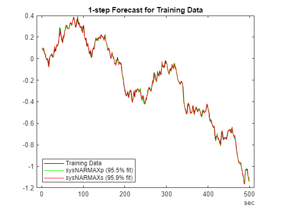
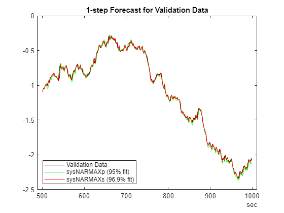
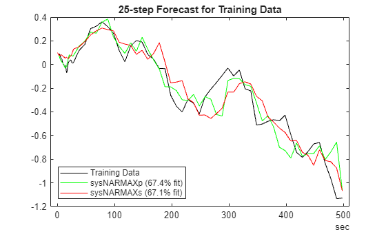
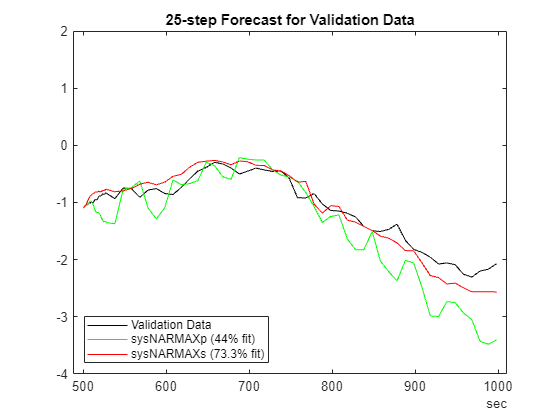
Assess the predictive abilities of these models for the horizons of 1 and 25.

H = 1;
% Training data
plotPredictions(H, TrainData, sysNARMAXp, sysNARMAXs);

Prediction started ...done.

% Validation data
plotPredictions(H, ValidateData, sysNARMAXp, sysNARMAXs);

Prediction started ...done.

Next, assess the quality for 25 steap-ahead prediction.

H = 25;
% Training data
plotPredictions(H, TrainData, sysNARMAXp, sysNARMAXs);

Prediction started ...done.

% Validation data
plotPredictions(H, ValidateData, sysNARMAXp, sysNARMAXs);

Prediction started ...done.

ylim([-4 2])

Using Neural State Space Models

Finally, we illustrate the creation of a predictive NARMAX model using Neural State-Space models. These models use deep networks from Deep Learning Toolbox™ to define the state-transition and the output functions of a nonlinear state-space model.

Define the following as model states:

$$X(k):=(\underset{}{\overset{\sim }{y}}(k-1),\underset{}{\overset{\sim }{y}}(k-2),y(k-1),y(k-2),u(k-1),u(k-2),u(k-3){)}^T$$. Using this state definition generate state data:

Reg = linearRegressor(["yp","y","u"],{1:2, 1:2, 1:3}); 
% Generate state data (NeuralStateSpace models require state measurements to be made directly
% available)
X = getreg(Reg, MultiInputTrainData);
X = X{4:end,:}; % omit rows affected by initial conditions
U = MultiInputTrainData;
U = U(4:end).u;

SSTrainData = iddata(X,U,1);
nx = 7; % there are 7 states
nu = 2; % there are 2 inputs

% Create a discrete-time Neural State Space model that uses 7 states and 2 inputs.
neuralSS_predict = idNeuralStateSpace(nx, NumInputs=nu, Ts=1);

% Create a 2-hidden-layer sigmoid state-transition network
net = createMLPNetwork(neuralSS_predict, "state", LayerSizes=[50 50], Activations="sigmoid");
neuralSS_predict.StateNetwork = net;

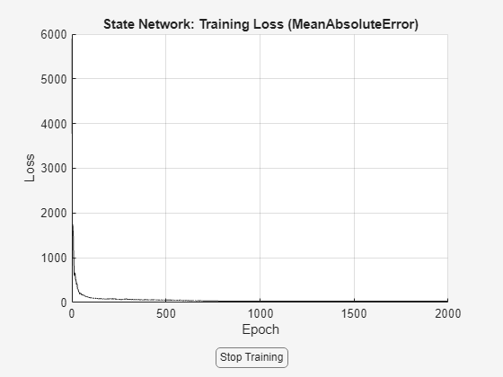
The NLSSEST command trains a neural state-space model. The training is always aimed at minimizing the simulation error, which is the goal here. For training the model, use the following setup:

• Use ADAM as the training method

• Segment the data into overlapping segments of length 50. Overlap length is 10 samples.

• Use a faster learning rate of 0.01 (the default is 0.001)

• Limit the number of training epochs to 2000

• Drop the learning rate by a factor of 0.1 every 700 epochs

% Prepare training options
nnOpt = nssTrainingOptions("ADAM");
nnOpt.WindowSize = 50;
nnOpt.Overlap = 10;
nnOpt.MaxEpochs = 2000;
nnOpt.LearnRate = 0.01;
nnOpt.LearnRateSchedule='piecewise';
nnOpt.LearnRateDropPeriod = 700;

% Train the model using the last data segment for in-training cross validation
rng(1)
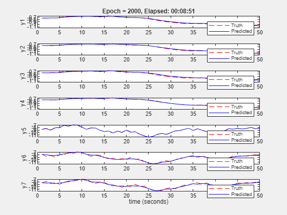
neuralSS_predict = nlssest(SSTrainData, neuralSS_predict, nnOpt, UseLastExperimentForValidation=true)

Generating estimation report...done.

neuralSS_predict =

Discrete-time Neural ODE in 7 variables
     x(t+1) = f(x(t),u(t))
       y(t) = x(t) + e(t)
 
f(.) network:
  Deep network with 2 fully connected, hidden layers
  Activation function: sigmoid
 
Variables: x1, x2, x3, x4, x5, x6, x7
Sample time: 1 seconds
 
Status:                                                             
Estimated using NLSSEST on time domain data "SSTrainData".          
Fit to estimation data: [95.97;96.69;95.53;97.37;99.38;94.38;93.27]%
MSE: 0.2108                                                         

Model Properties

Similarlly, we can directly train a response simulator. For training a simulator, we don't need to create an extended dataset.

Reg = linearRegressor(["y","u"],{1:3, 1:3}); 
X = getreg(Reg, TT);
nx = width(X);
X = X{4:end,:}; % omit rows affected by initial conditions
U = TT.u(4:end);
AllData = iddata(X,U,1,OutputName=["y","x"+(2:nx)],InputName="u");
SSTrainData_sim = AllData(1:500);
SSValData_sim = AllData(501:end);

nu = 1; % there is only 1 input

% Create a discrete-time Neural State Space model that uses 7 states and 2 inputs.
neuralSS_sim = idNeuralStateSpace(nx, NumInputs=nu, Ts=1);

% Create a 2-hidden-layer  state-transition network
net = createMLPNetwork(neuralSS_sim, "state", LayerSizes=[64 64], Activations="sigmoid");
neuralSS_sim.StateNetwork = net;
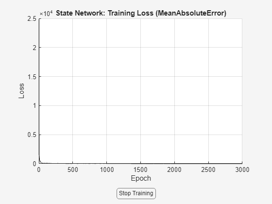
nnOpt.LearnRateDropPeriod = 1000;
nnOpt.MaxEpochs = 3000;
nnOpt.LearnRate = 0.1;

rng(1)
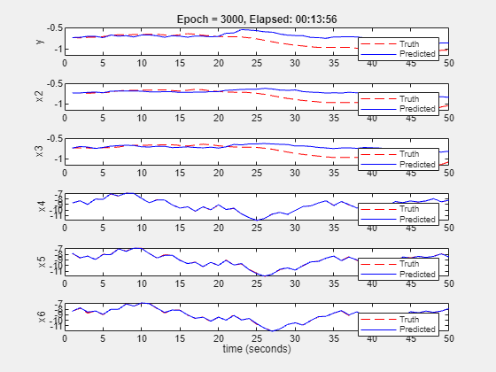
neuralSS_sim = nlssest(SSTrainData_sim, neuralSS_sim, nnOpt, UseLastExperimentForValidation=true)

Generating estimation report...done.

neuralSS_sim =

Discrete-time Neural ODE in 6 variables
     x(t+1) = f(x(t),u(t))
       y(t) = x(t) + e(t)
 
f(.) network:
  Deep network with 2 fully connected, hidden layers
  Activation function: sigmoid
 
Variables: x1, x2, x3, x4, x5, x6
Sample time: 1 seconds
 
Status:                                                       
Estimated using NLSSEST on time domain data "SSTrainData_sim".
Fit to estimation data: [74.7;76.09;76.28;99.56;99.31;99.05]% 
MSE: 0.02943                                                  

Model Properties

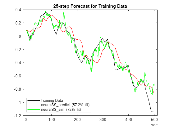
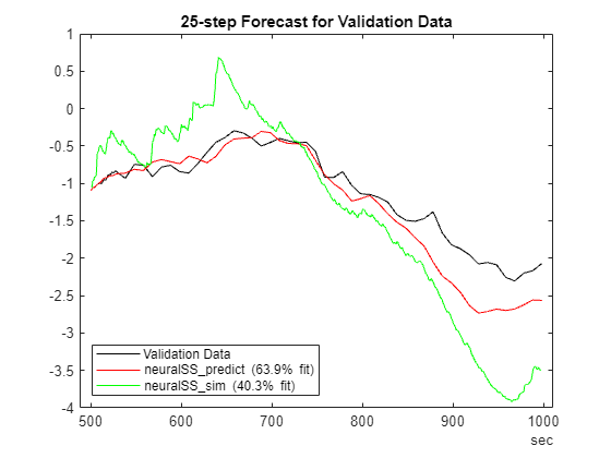
Use the model for predicting 25 steps into the future. Do so for both the training and the validation dataset.

H = 25;
% Training data
plotPredictions(H, TrainData, neuralSS_predict);

Prediction started ...done.

hold on
yp = predict(neuralSS_sim, SSTrainData_sim, H); yp=yp.y;
FitPercent = (1-goodnessOfFit(SSTrainData_sim.y(:,1), yp(:,1), 'nrmse'))*100

FitPercent = 
72.0295

p = plot(SSTrainData_sim.SamplingInstants,yp(:,1),'g');
p.DisplayName = sprintf('neuralSS\\_sim (%2.3g%% fit)',FitPercent);
hold off

% Validation data
plotPredictions(H, ValidateData, neuralSS_predict);

Prediction started ...done.

hold on
ypv = predict(neuralSS_sim, SSValData_sim, H); ypv=ypv.y;
FitPercent = (1-goodnessOfFit(SSValData_sim.y(:,1), ypv(:,1), 'nrmse'))*100

FitPercent = 
40.2620

p = plot(SSValData_sim.SamplingInstants,ypv(:,1),'g');
p.DisplayName = sprintf('neuralSS\\_sim (%2.3g%% fit)',FitPercent);
hold off

Simulation Capability

Finally, let us compare the simulation ability (that is, forecast infinitely into future) of the trained models.

% Set the prediction horizon to Inf. In practice it means forecasting to the length of the available data.
% For ValidationData, this implies a horizon of 500.
H = Inf;
plotPredictions(H, ValidateData, ...
   sysARMAX, ... linear ARMAX model
   sysNARX, ... nonlinear ARX model (no MA term)
   sysNARMAXp,... nonlinear ARMAX trained to minimize 1-step prediction error
   sysNARMAXs,...nonlinear ARMAX trained to minimize simulation error
   sysGrey,... nonlinear ARX + additive linear MA model
   neuralSS_predict... neural state-space model trained to minimize 1-step prediction error
   );

Prediction started ...done.
Prediction started ...done.
Prediction started ...done.

ylim([-4 2])

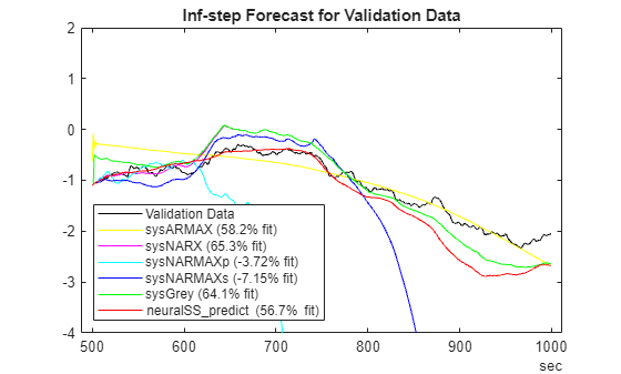
As been, forecasting indefinitely into future is a demanding goal for models of NARMAX processes.

Conclusions

Going from an NARX to a NARMAX model means that the 1-step-ahead response predictor becomes recursive (see predictNARMAX) and hence takes longer to compute the results. But the benefit is that the (one-step) predictions are more accurate for systems whose output measurement depends upon not just the present but also the past disturbances.

A recipe for creating a NARMAX model with additive moving average terms consists of the following steps:

1. Fit a NARX model to the data using the NLARX command.

2. Compute the model residuals using the PE or RESID command.

3. Fit a linear moving-average (MA) model to the residuals (use ARMAX command with na=0, nc = MA order)

4. "Combine" the NARX model with the linear MA model using the grey-box modeling approach (see idnlgrey, nlgreyest). Refine the free coefficients of the resulting grey-box model in order to improve the fit to the data.

For more generic/direct modeling of a time-series as a NARMAX process, with no additional simplifying assumptions regarding the nature of the contribution of the disturbances, you can use the following recipe:

1. Create an extended model structure that uses two input sets - one corresponding to the measured outputs and second one corresponding to the measured exogenous inputs. Suppose measured outputs are called $$y_{meas}$$, and the measured exogenous inputs are called $$u$$. Then the inputs of the extended model are $$(y_{meas}(k),u(k))$$, while its output is the (1-step-ahead) predicted response $$\underset{}{\overset{\sim }{y}}(k)$$.

2. Prepare training data that uses samples of $$y_{meas}$$ as output and the samples of $$(y_{meas},u)$$ as inputs. Note that $$y_{meas}$$ is being used both as the output time series as well as the exogenous input in this training dataset.

3. Train any suitable model structure for which the training algorithm is capable of minimizing simulation errors. This includes Nonlinear ARX models (with Focus="simulation"), Nonlinear State Space models, Nonlinear Grey-Box models, and Hammerstein-Wiener models; for the latter three structures, the training focus is always "simulation".

4. Use a specialized multi-step-ahead prediction method (such as predictNARMAX) for using the model for forecasting the future outcomes.

Alternatively, directly train a nonlinear model for simulation fidelity (models sysNARMAXs and neuralSS_sim in this example). Such a model can be used for finite-horizon prediction too, although it will have no mechanism for correcting the predictions based on most recent output measurements.