Leaving feedback is a two-step process. At the bottom of most pages in the MATLAB documentation is a star rating.
Start by selecting a star that best answers the question. After selecting a star rating, an edit box appears where you can offer specific feedback.
When you press "Submit" you'll see the confirmation dialog below. You cannot go back and edit your content, although you can refresh the page to go through that process again.
Tips on leaving feedback
Be productive. The reader should clearly understand what action you'd like to see, what was unclear, what you think needs work, or what areas were really helpful.
Positive feedback is also helpful. By nature, feedback often focuses on suggestions for changes but it also helps to know what was clear and what worked well.
Point to specific areas of the page. This helps the reader to narrow the focus of the page to the area described by your feedback.
What happens to that feedback?
Before working at MathWorks I often left feedback on documentation pages but I never knew what happens after that. One day in 2021 I shared my speculation on the process:
> That feedback is received by MathWorks Gnomes which are never seen nor heard but visit the MathWorks documentation team at night while they are sleeping and whisper selected suggestions into their ears to manipulate their dreams. Occassionally this causes them to wake up with a Eureka moment that leads to changes in the documentation.
I'd like to let you in on the secret which is much less fanciful. Feedback left in the star rating and edit box are collected and periodically reviewed by the doc writers who look for trends on highly trafficked pages and finer grain feedback on less visited pages. Your feedback is important and often results in improvements.
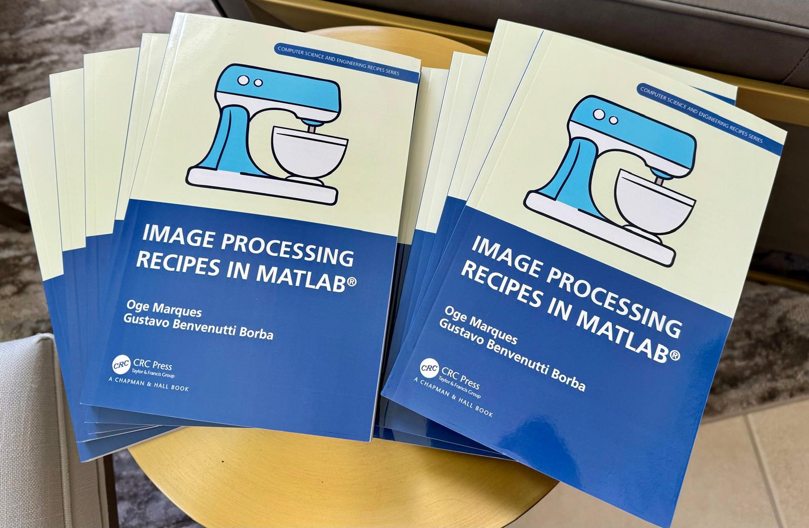
📚 New Book Announcement: "Image Processing Recipes in MATLAB" 📚
I am delighted to share the release of my latest book, "Image Processing Recipes in MATLAB," co-authored by my dear friend and colleague Gustavo Benvenutti Borba.
This 'cookbook' contains 30 practical recipes for image processing, ranging from foundational techniques to recently published algorithms. It serves as a concise and readable reference for quickly and efficiently deploying image processing pipelines in MATLAB.
Gustavo and I are immensely grateful to the MathWorks Book Program for their support. We also want to thank Randi Slack and her fantastic team at CRC Press for their patience, expertise, and professionalism throughout the process.
A colleague said that you can search the Help Center using the phrase 'Introduced in' followed by a release version. Such as, 'Introduced in R2022a'. Doing this yeilds search results specific for that release.
You can access any of the data available on the site as per the Alpha Vantage documentation using these two lines of code but with different designations for the requested data as per the documentation.
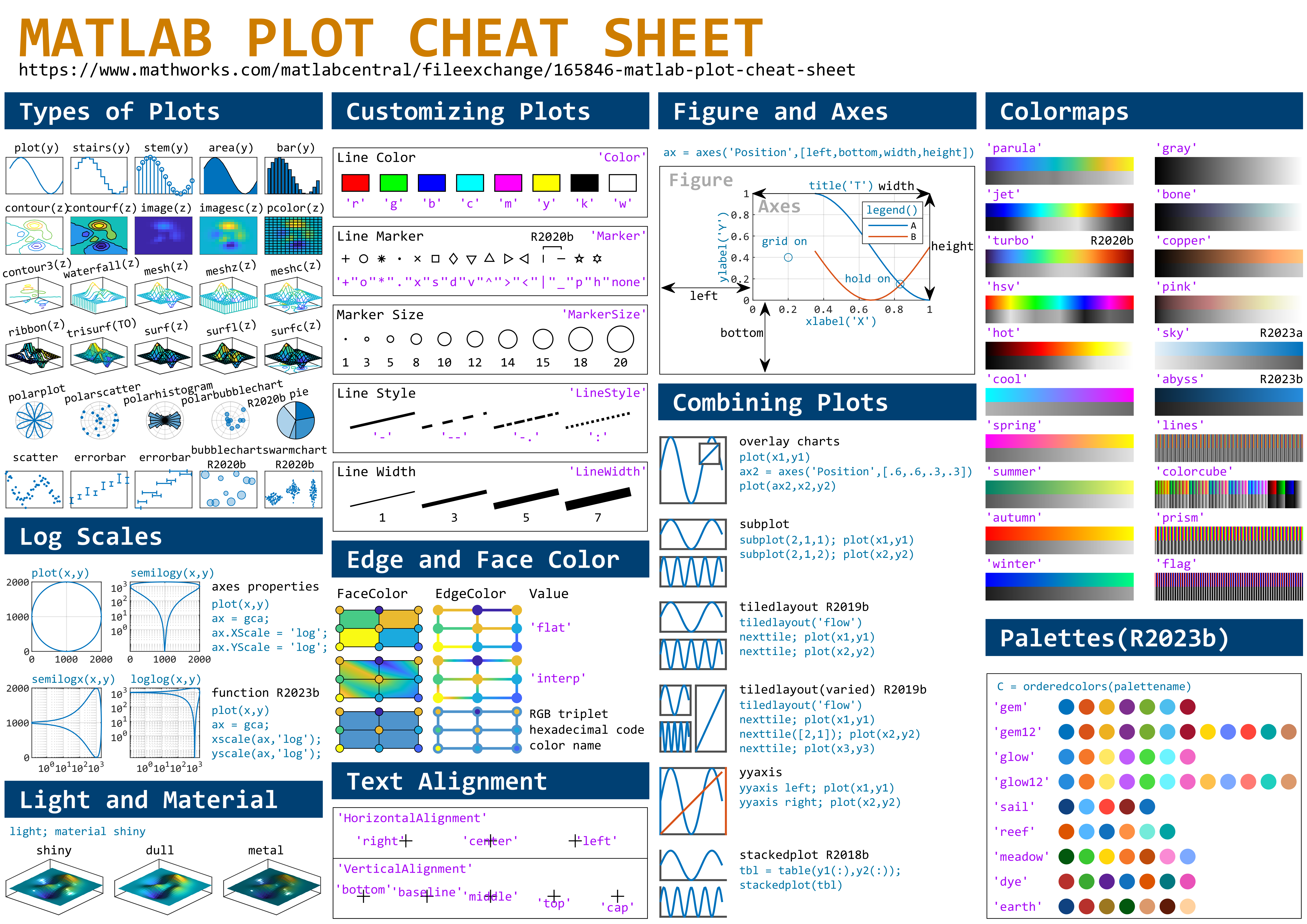
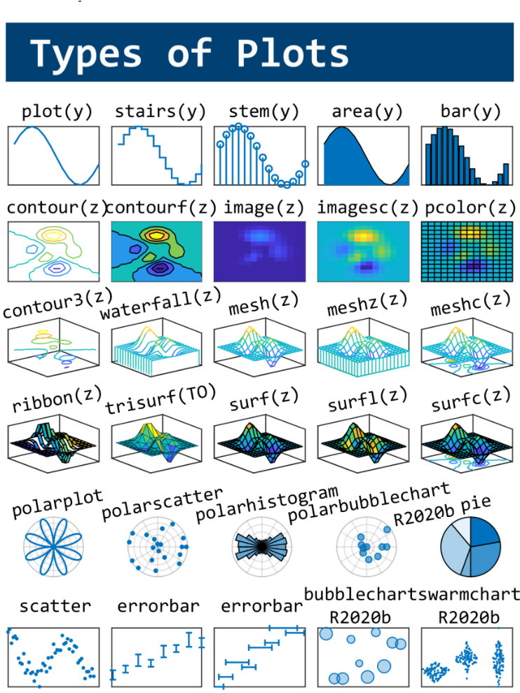
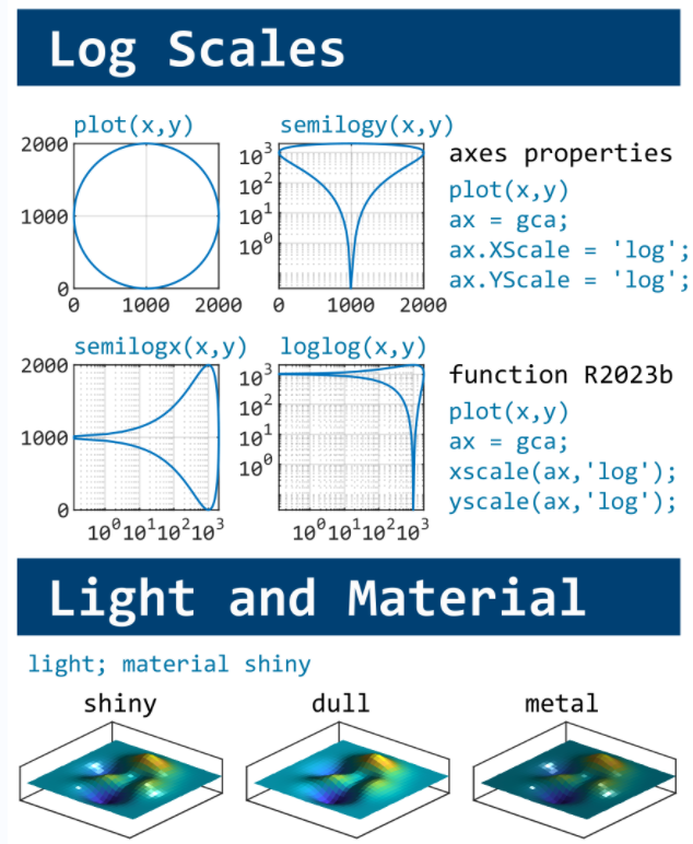
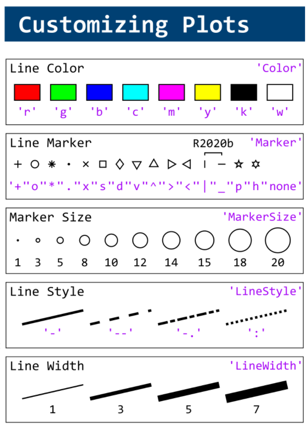
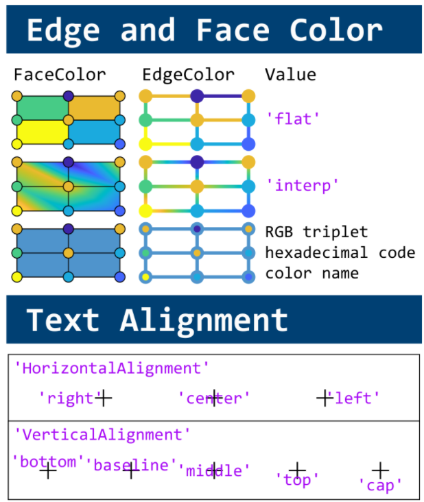
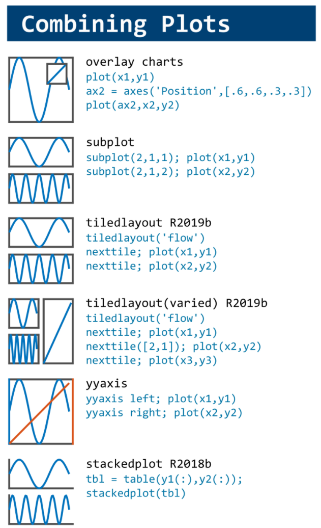
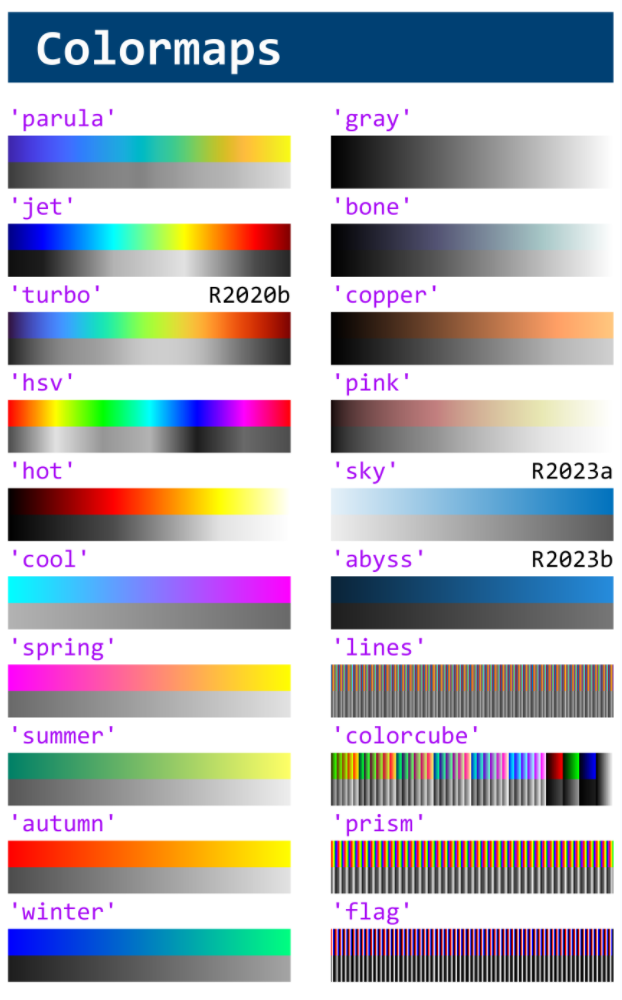
MATLAB used to have official visualization-cheat-sheet, but there have been quite a few new updates in MATLAB versions recently. Therefore, I made my own cheat sheet and marked the versions of each new thing that were released :
I believe many of you have been captivated by the innovative entries from Zhaoxu Liu / slanderer, in the 2023 MATLAB Flipbook Mini Hack contest.
Ever wondered about the person behind these creative entries? What drives a MATLAB user to such levels of skill? And what inspired his participation in the contest? We were just as curious as you are!
We were delighted to catch up with him and learn more about his use of MATLAB. The interview has recently been published in MathWorks Blogs. For an in-depth look into his insights and experiences, be sure to read our latest blog post: Community Q&A – Zhaoxu Liu.
But the conversation doesn't end here! Who would you like to see featured in our next interview? Drop their name in the comments section below and let us know who we should reach out to next!
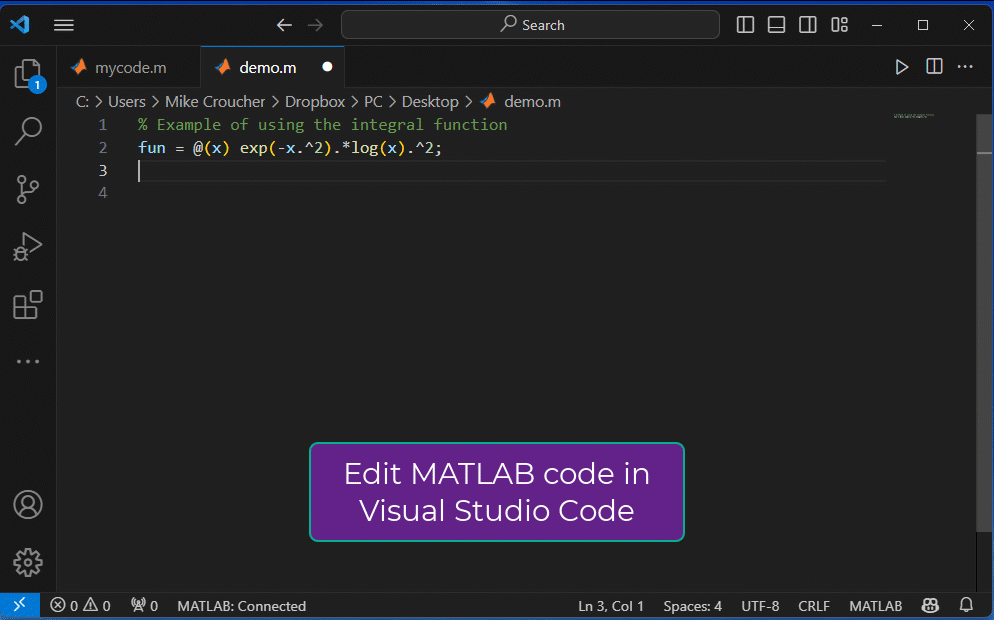
Temporary print statements are often helpful during debugging but it's easy to forget to remove the statements or sometimes you may not have writing privileges for the file. This tip uses conditional breakpoints to add print statements without ever editing the file!
What are conditional breakpoints?
Conditional breakpoints allow you to write a conditional statement that is executed when the selected line is hit and if the condition returns true, MATLAB pauses at that line. Otherwise, it continues.
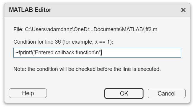
The Hack: use ~fprintf() as the condition
fprintf prints information to the command window and returns the size of the message in bytes. The message size will always be greater than 0 which will always evaluate as true when converted to logical. Therefore, by negating an fprintf statement within a conditional breakpoint, the fprintf command will execute, print to the command window, and evalute as false which means the execution will continue uninterupted!
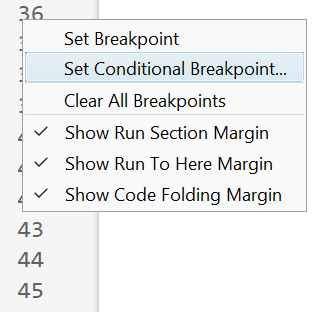
How to set a conditional break point
1. Right click the line number where you want the condition to be evaluated and select "Set Conditional Breakpoint"
2. Enter a valid MATLAB expression that returns a logical scalar value in the editor dialog.
Handy one-liners
Check if a line is reached: Don't forget the negation (~) and the line break (\n)!
~fprintf('Entered callback function\n')
Display the call stack from the break point line: one of my favorites!
Make sense of frequent hits: In some situations such as responses to listeners or interactive callbacks, a line can be executed 100s of times per second. Incorporate a timestamp to differentiate messages during rapid execution.
This tip not only keeps your code clean but also offers a dynamic way to monitor code execution and variable states without permanent modifications. Interested in digging deeper? @Steve Eddins takes this tip to the next level with his Code Trace for MATLAB tool available on the File Exchange (read more).
I am excited to announce that I am currently working on a book project centered around Matrix Algebra, specifically designed for MATLAB users. This book aims to cater to undergraduate students in engineering, where Matrix Algebra serves as a foundational element.
Matrix Algebra is not only pivotal in understanding complex engineering concepts but also in applying these principles effectively in various technological solutions. MATLAB, renowned for its powerful computational capabilities, is an excellent tool to explore and implement these concepts, making it a perfect companion for this book.
As I embark on this journey to create a resource that bridges theoretical matrix algebra with practical MATLAB applications, I am looking for one or two knowledgeable individuals who have a firm grasp of both subjects. If you have experience in teaching or applying matrix algebra in engineering contexts and are familiar with MATLAB, your contribution could be invaluable.
Collaborators will help in shaping the content to ensure it is educational, engaging, and technically robust, making complex concepts accessible and applicable for students.
If you are interested in contributing to this project or know someone who might be, please reach out to discuss how we can work together to make this book a valuable resource for engineering students.
Thank you and looking forward to your participation!
You can download these toolkits from the provided links.
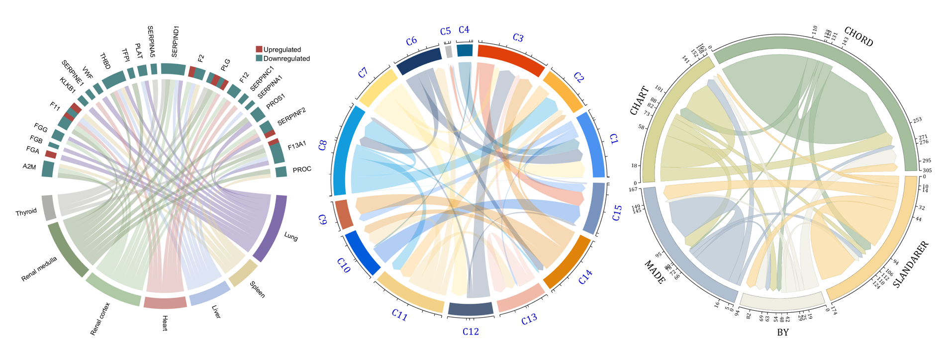
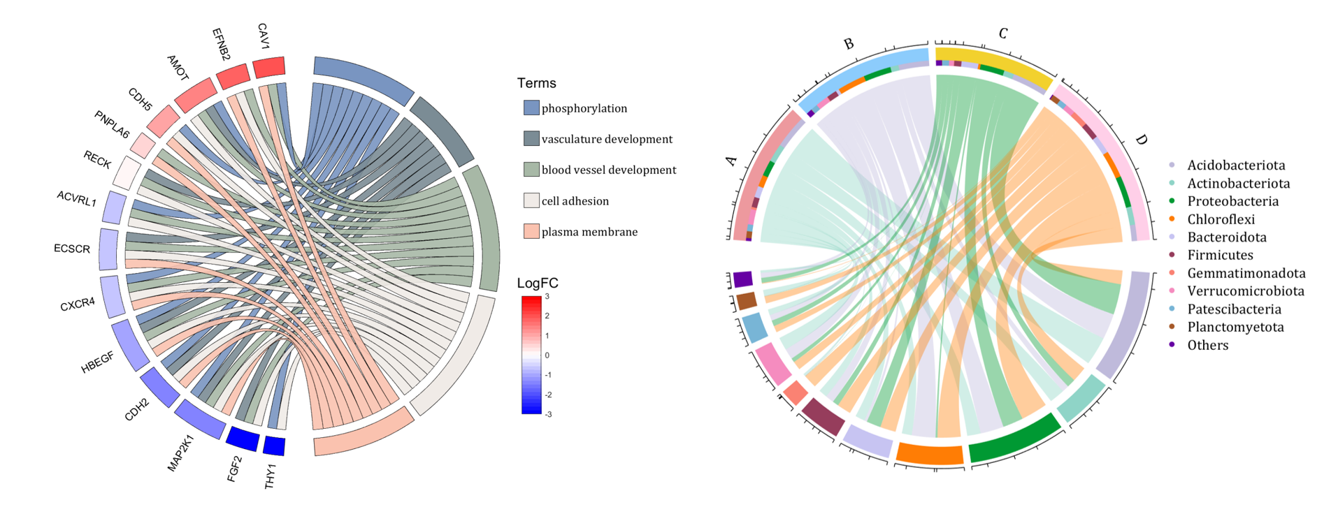
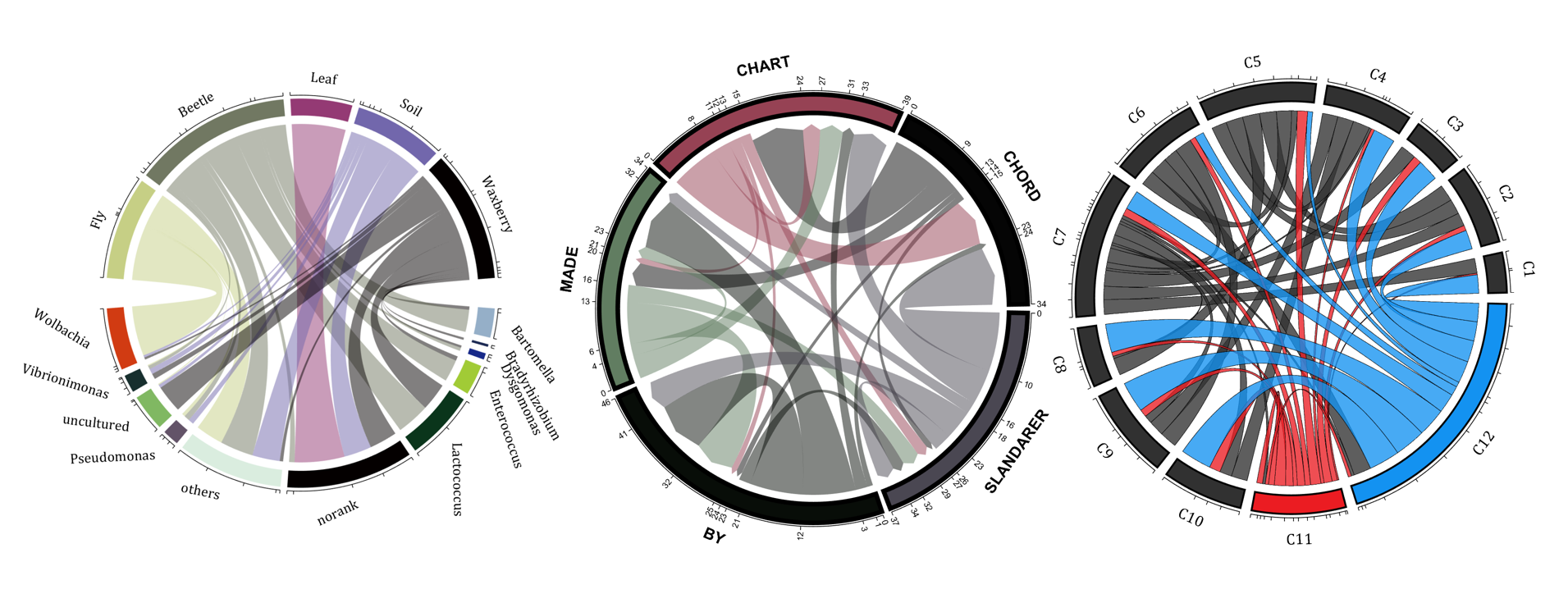
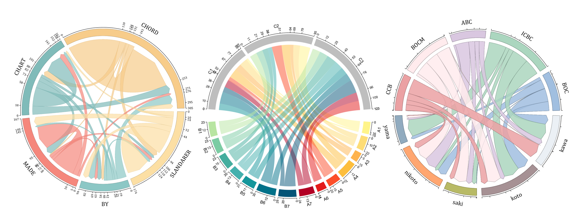
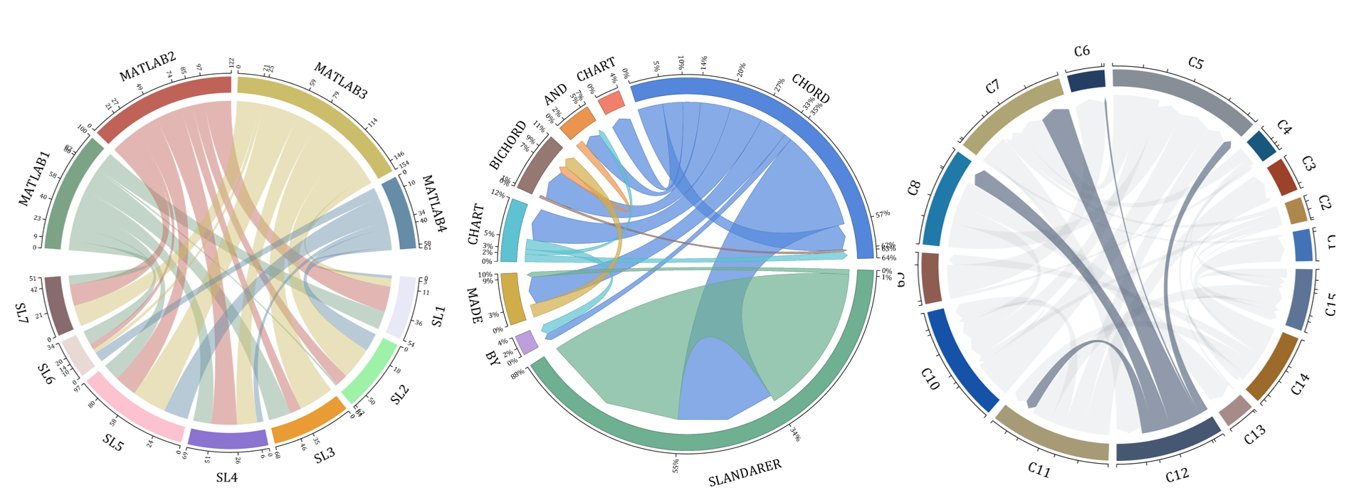
The reason for writing this article is that many people have started using the chord diagram plotting toolkit that I developed. However, some users are unsure about customizing certain styles. As the developer, I have a good understanding of the implementation principles of the toolkit and can apply it flexibly. This has sparked the idea of challenging myself to create various styles of chord diagrams. Currently, the existing code is quite lengthy. In the future, I may integrate some of this code into the toolkit, enabling users to achieve the effects of many lines of code with just a few lines.
Without further ado, let's see the extent to which this MATLAB toolkit can currently perform.
I feel like no one at UC San Diego knows this page, let alone this server, is still live. For the younger generation, this is what the whole internet used to look like :)
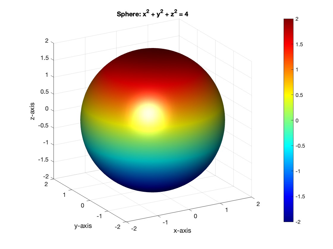
To solve a surface integral for example the over the sphere easily in MATLAB, you can leverage the symbolic toolbox for a direct and clear solution. Here is a tip to simplify the process:
Use Symbolic Variables and Functions: Define your variables symbolically, including the parameters of your spherical coordinates θ and ϕ and the radius r . This allows MATLAB to handle the expressions symbolically, making it easier to manipulate and integrate them.
Express in Spherical Coordinates Directly: Since you already know the sphere's equation and the relationship in spherical coordinates, define x, y, and z in terms of r , θ and ϕ directly.
Perform Symbolic Integration: Use MATLAB's `int` function to integrate symbolically. Since the sphere and the function are symmetric, you can exploit these symmetries to simplify the calculation.
Here’s how you can apply this tip in MATLAB code:
% Include the symbolic math toolbox
syms theta phi
% Define the limits for theta and phi
theta_limits = [0, pi];
phi_limits = [0, 2*pi];
% Define the integrand function symbolically
integrand = 16 * sin(theta)^3 * cos(phi)^2;
% Perform the symbolic integral for the surface integral
I am often talking to new MATLAB users. I have put together one script. If you know how this script works, why, and what each line means, you will be well on your way on your MATLAB learning journey.
% Clear existing variables and close figures
clear;
close all;
% Print to the Command Window
disp('Hello, welcome to MATLAB!');
% Create a simple vector and matrix
vector = [1, 2, 3, 4, 5];
matrix = [1, 2, 3; 4, 5, 6; 7, 8, 9];
% Display the created vector and matrix
disp('Created vector:');
disp(vector);
disp('Created matrix:');
disp(matrix);
% Perform element-wise multiplication
result = vector .* 2;
% Display the result of the operation
disp('Result of element-wise multiplication of the vector by 2:');
disp(result);
% Create plot
x = 0:0.1:2*pi; % Generate values from 0 to 2*pi
y = sin(x); % Calculate the sine of these values
% Plotting
figure; % Create a new figure window
plot(x, y); % Plot x vs. y
title('Simple Plot of sin(x)'); % Give the plot a title
xlabel('x'); % Label the x-axis
ylabel('sin(x)'); % Label the y-axis
grid on; % Turn on the grid
disp('This is the end of the script. Explore MATLAB further to learn more!');
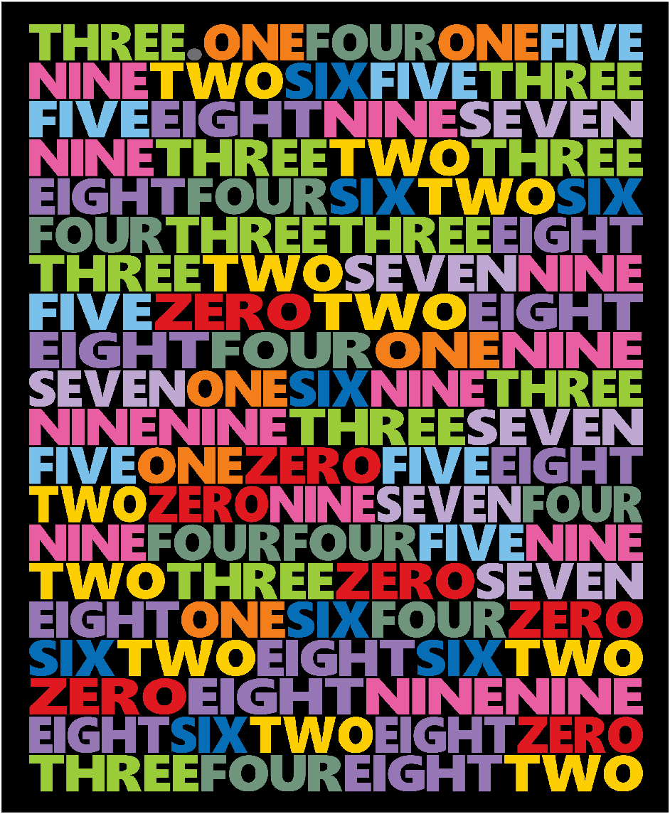
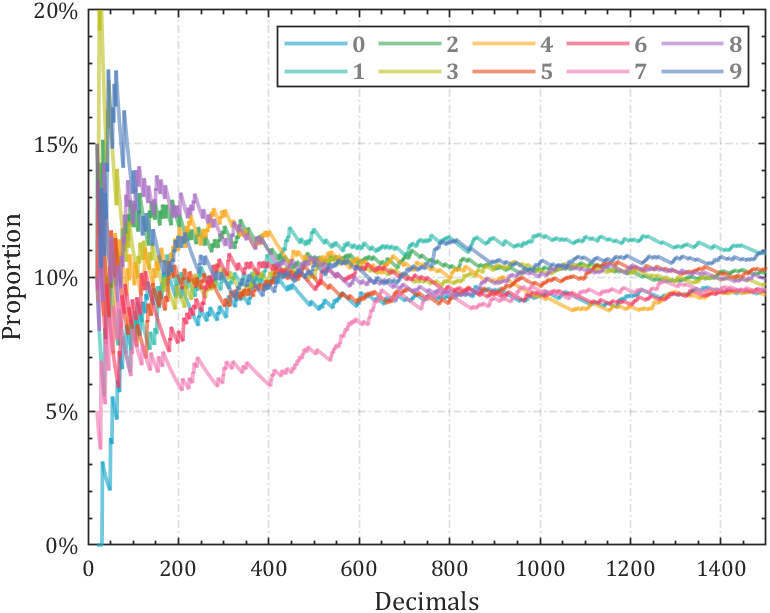
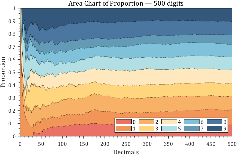
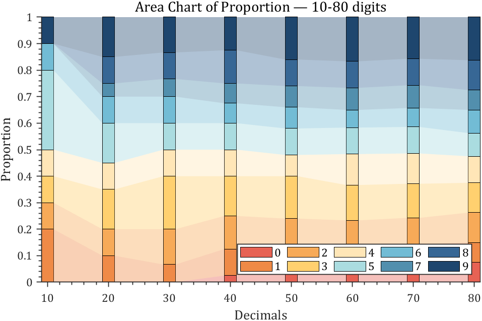
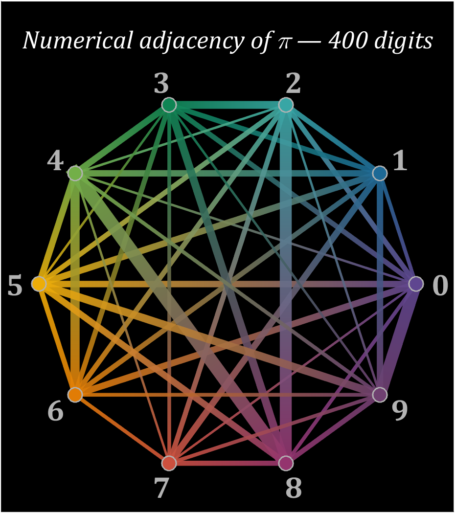
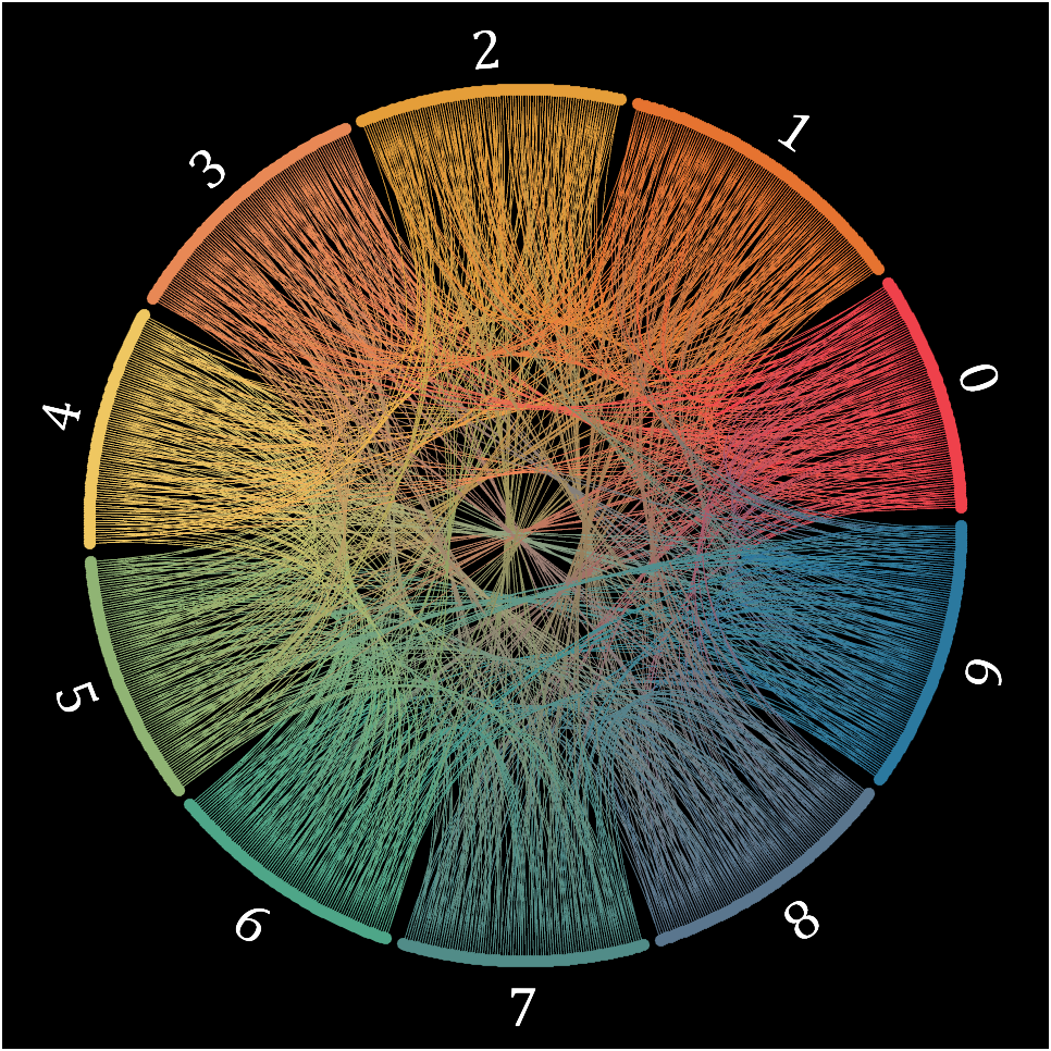
Firstly, in order to obtain the first n decimal places of pi, we need to write the following code (to prevent inaccuracies, we need to take a few more tails and perform another operation of taking the first n decimal places when needed):
function Pi=getPi(n)
if nargin<1,n=3;end
Pi=char(vpa(sym(pi),n+10));
Pi=abs(Pi)-48;
Pi=Pi(3:n+2);
end
With this function to obtain the decimal places of pi, our visualization journey has begun~Step by step, from simple to complex~(Please try to use newer versions of MATLAB to run, at least R17b)
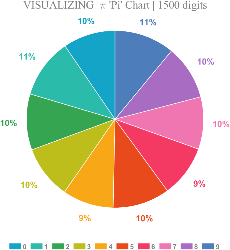
1 Pie chart
Just calculate the proportion of each digit to the first 1500 decimal places:
Imagine each decimal as a small ball with a mass of
For example, if, the weight of ball 0 is 1, ball 9 is 1.2589, the initial velocity of the ball is 0, and it is attracted by other balls. Gravity follows the inverse square law, and if the balls are close enough, they will collide and their value will become
After adding, take the mod, add the velocity direction proportionally, and recalculate the weight.
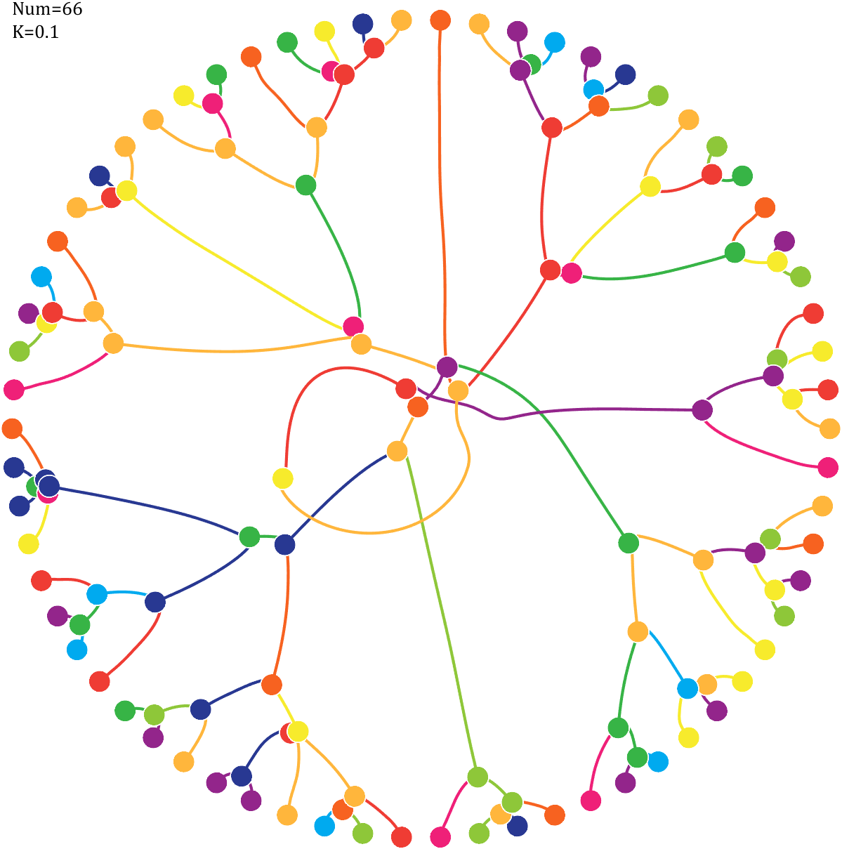
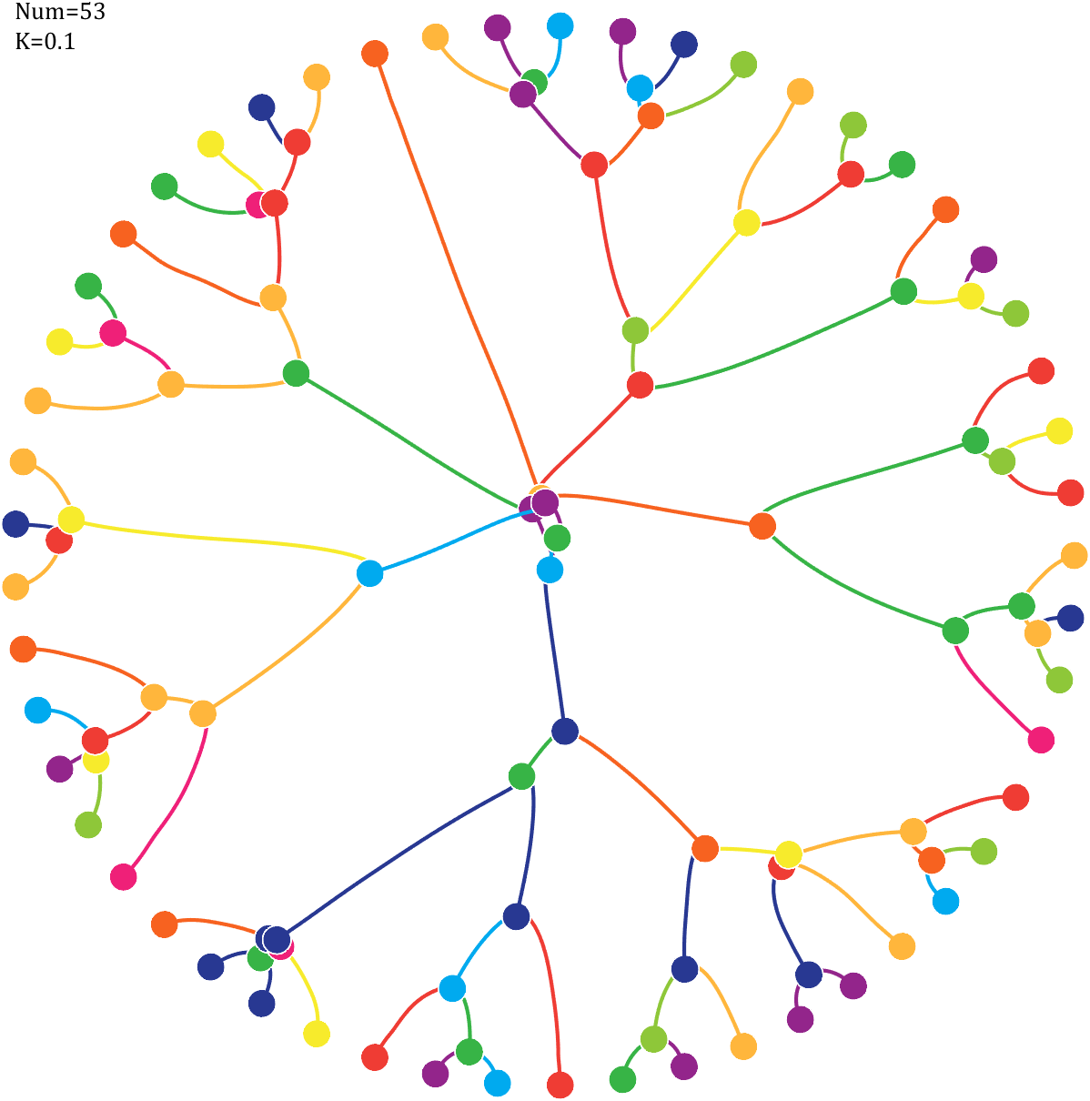
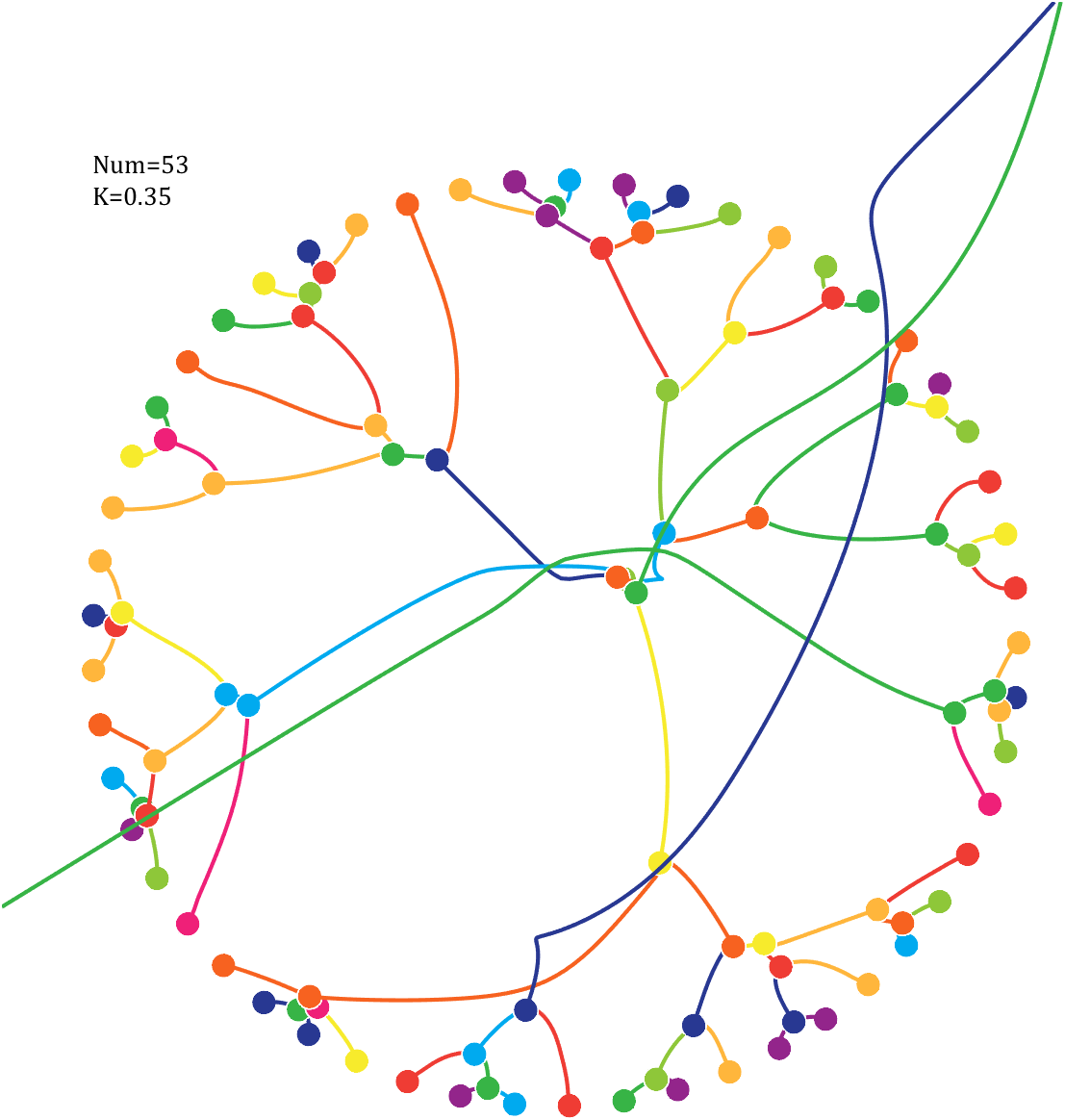
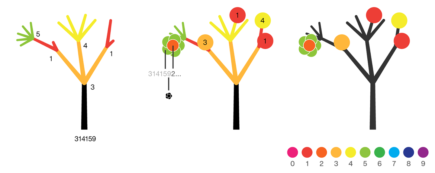
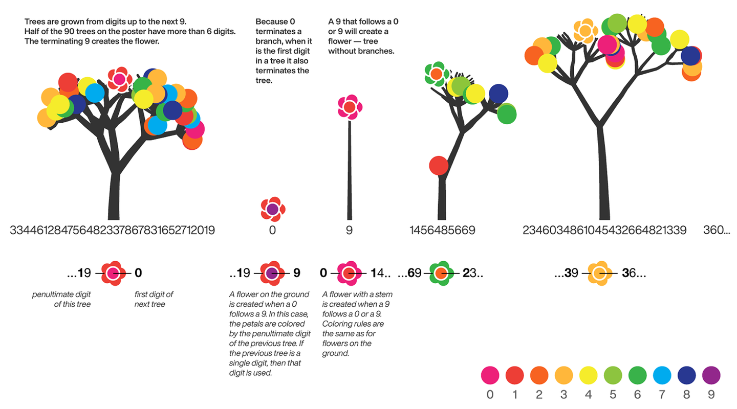
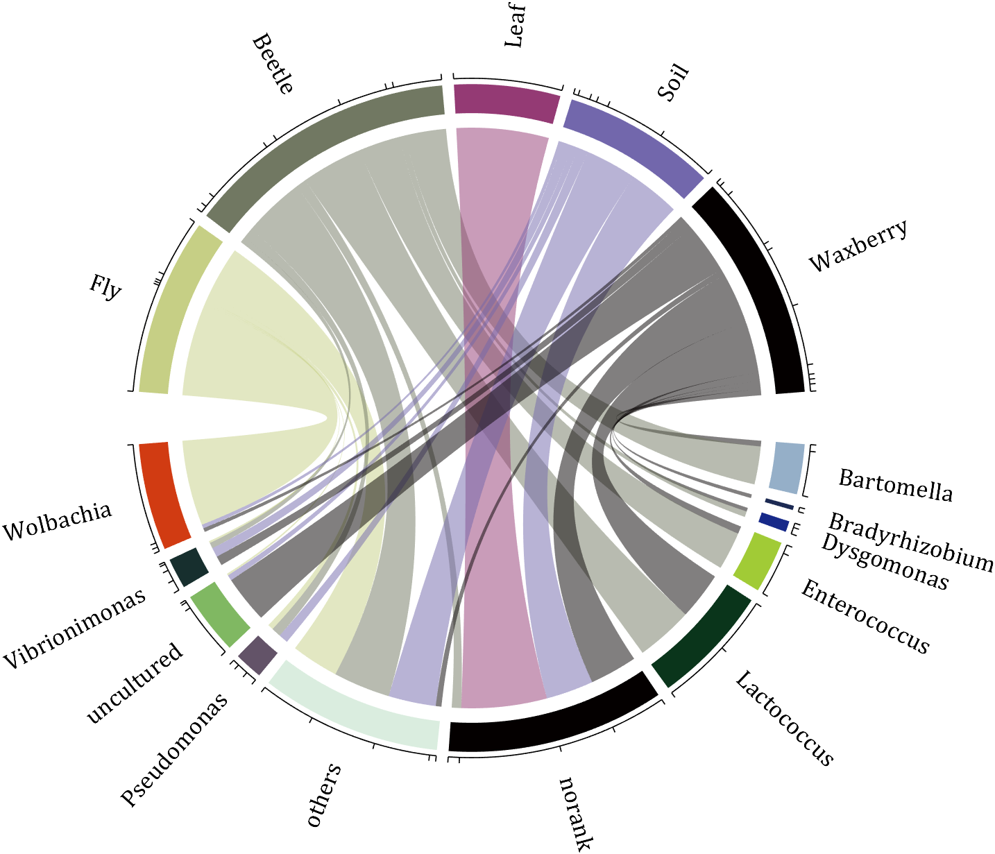
The digits of π are shown as a forest. Each tree in the forest represents the digits of π up to the next 9. The first 10 trees are "grown" from the digit sets 314159, 2653589, 79, 3238462643383279, 50288419, 7169, 39, 9, 3751058209, and 749.
BRANCHES
The first digit of a tree controls how many branches grow from the trunk of the tree. For example, the first tree's first digit is 3, so you see 3 branches growing from the trunk.
The next digit's branches grow from the end of a branch of the previous digit in left-to-right order. This process continues until all the tree's digits have been used up.
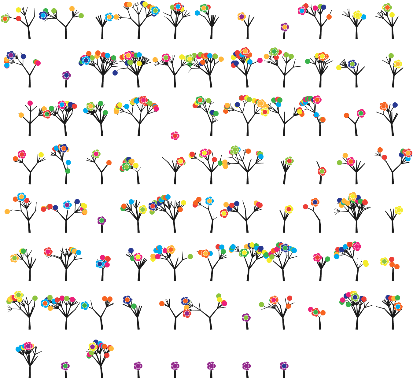
Each tree grows from a set of consecutive digits sampled from the digits of π up to the next 9. The first tree, shown here, grows from 314159. Each of the digits determine how many branches grow at each fork in the tree — the branches here are colored by their corresponding digit to illustrate this. Leaves encode the digits in a left-to-right order. The digit 9 spawns a flower on one of the branches of the previous digit. The branching exception is 0, which terminates the current branch — 0 branches grow!
LEAVES AND FLOWERS
The tree's digits themselves are drawn as circular leaves, color-coded by the digit.
The leaf exception is 9, which causes one of the branches of the previous digit to sprout a flower! The petals of the flower are colored by the digit before the 9 and the center is colored by the digit after the 9, which is on the next tree. This is how the forest propagates.
The colors of a flower are determined by the first digit of the next tree and the penultimate digit of the current tree. If the current tree only has one digit, then that digit is used. Leaves are placed at the tips of branches in a left-to-right order — you can "easily" read them off. Additionally, the leaves are distributed within the tree (without disturbing their left-to-right order) to spread them out as much as possible and avoid overlap. This order is deterministic.
The leaf placement exception are the branch set that sprouted the flower. These are not used to grow leaves — the flower needs space!
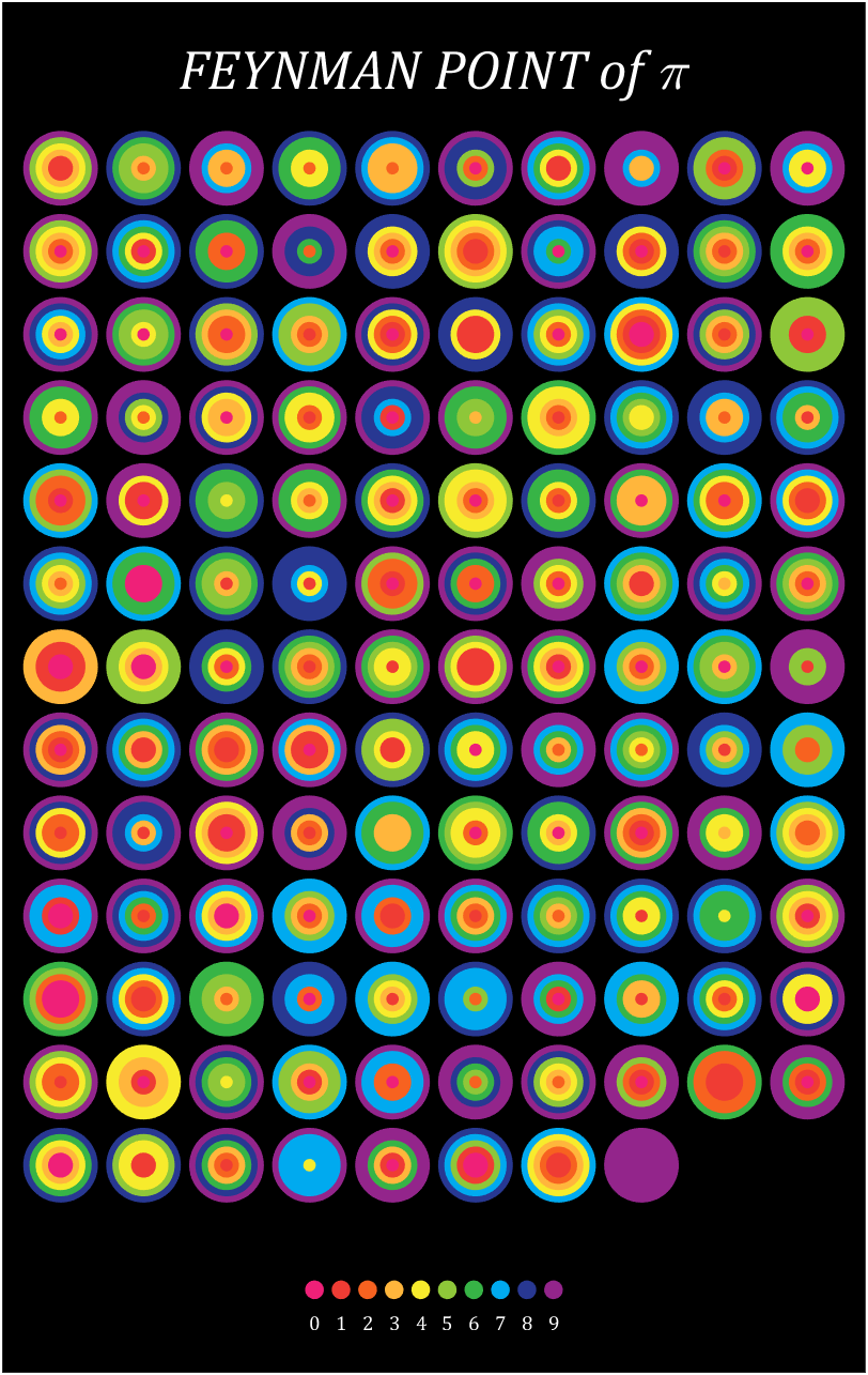
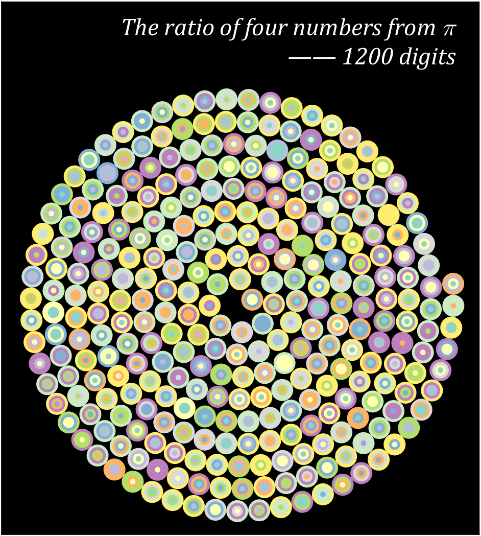
Let's still put the numbers in the form of circles, but the difference is that six numbers are grouped together, and the pure purple circle at the end is the six 9s that we are familiar with decimal places 762-767
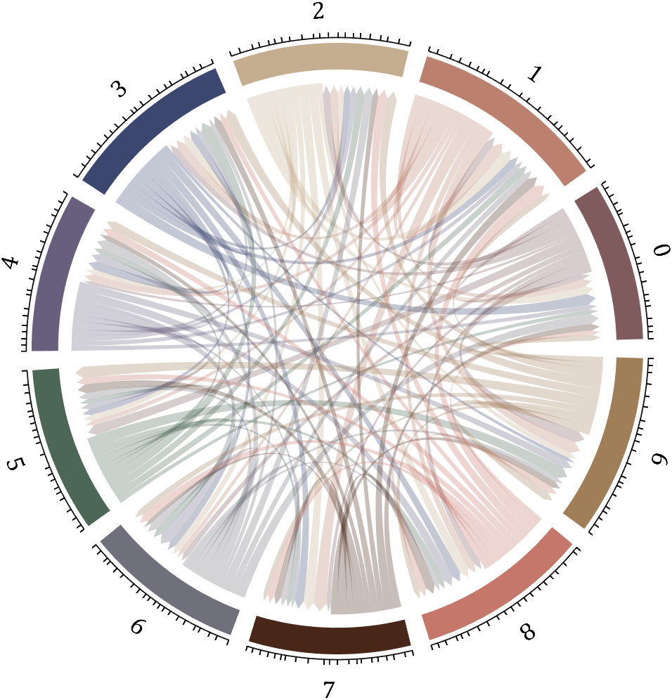
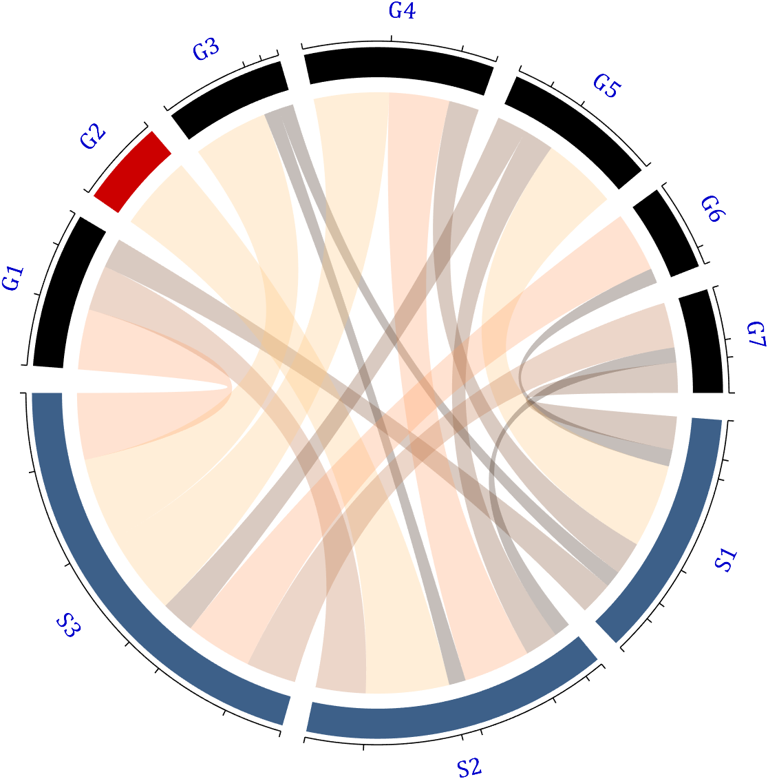
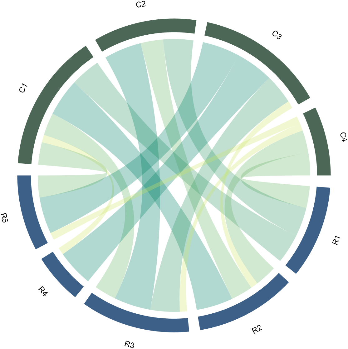
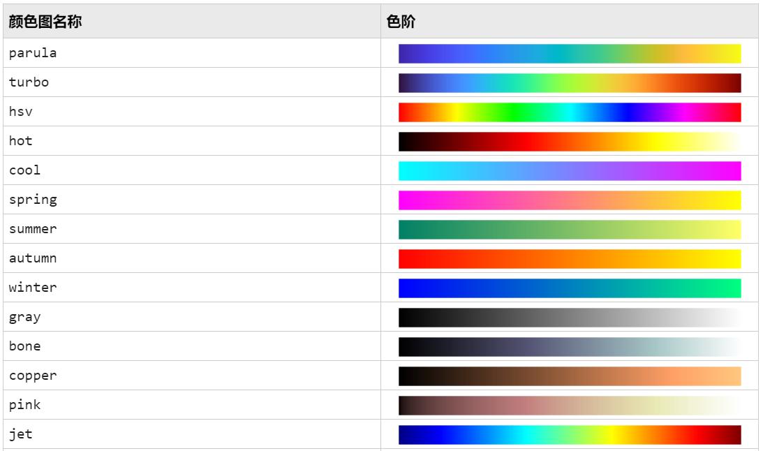
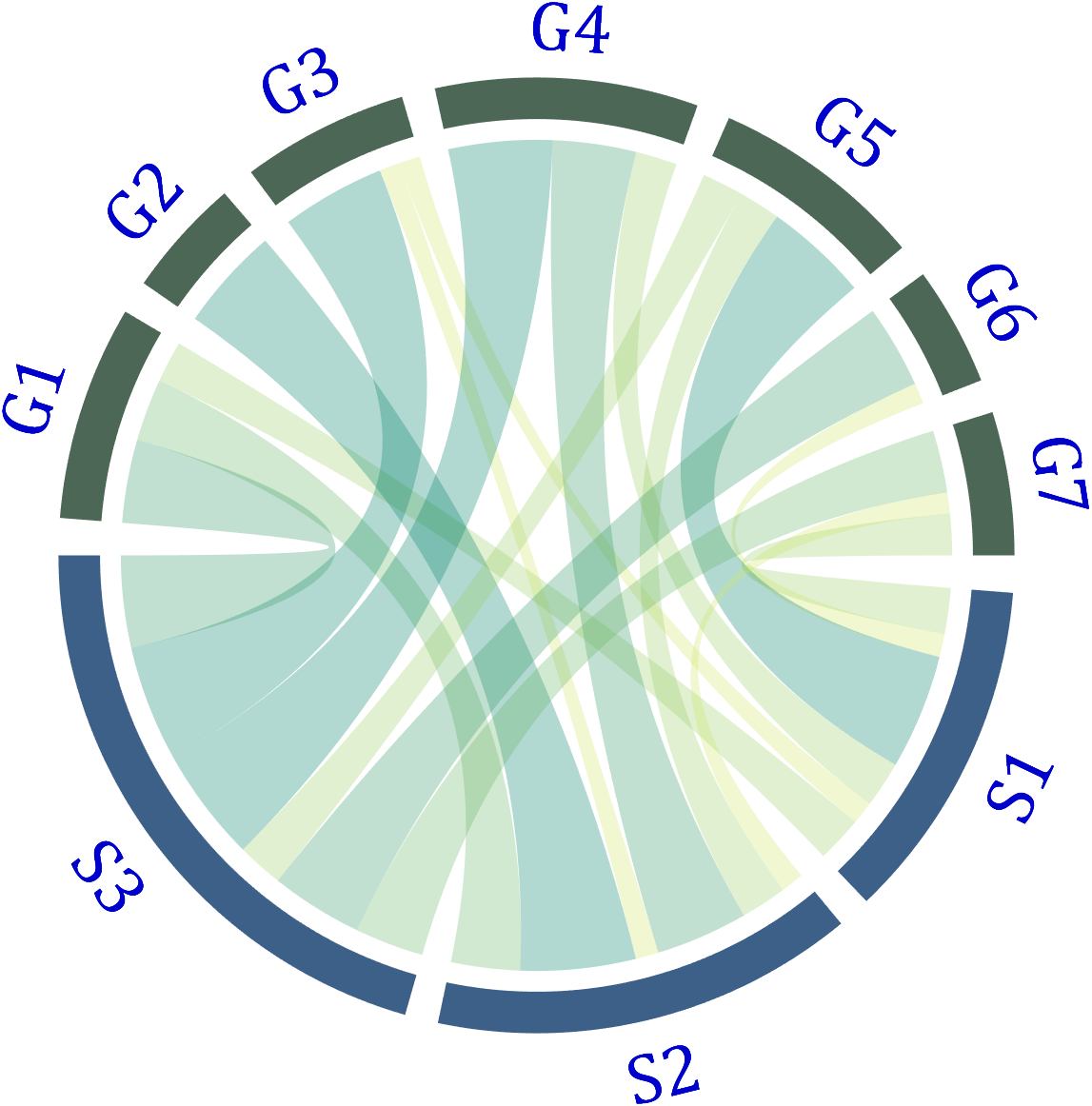
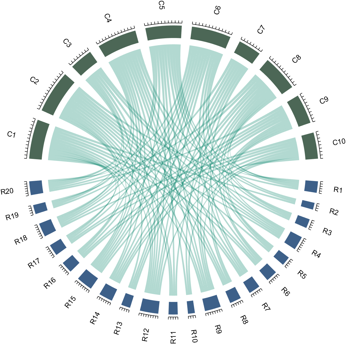
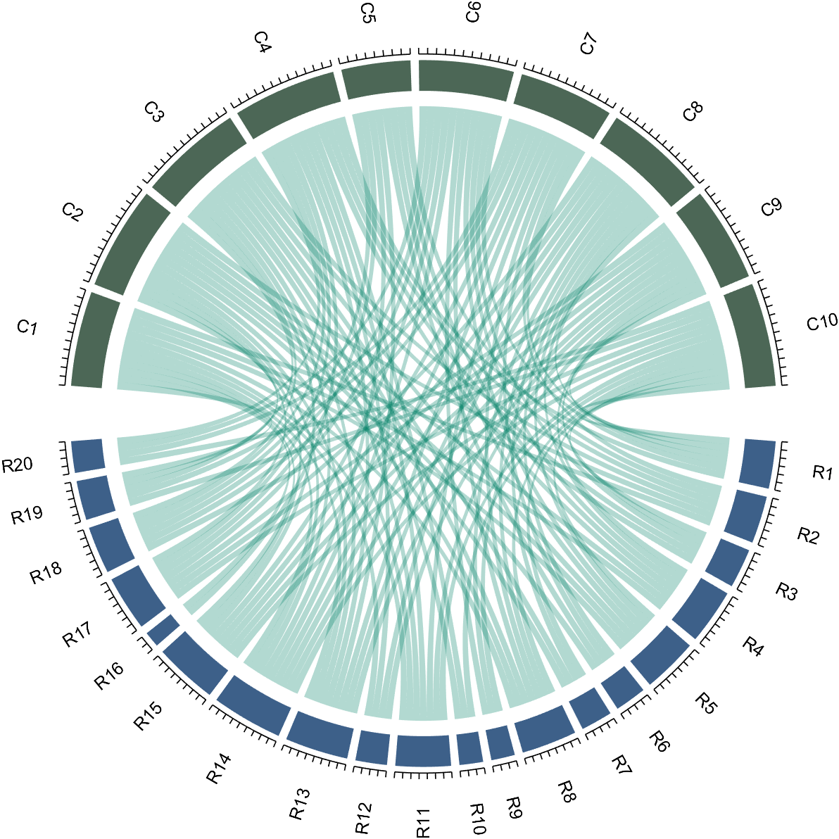
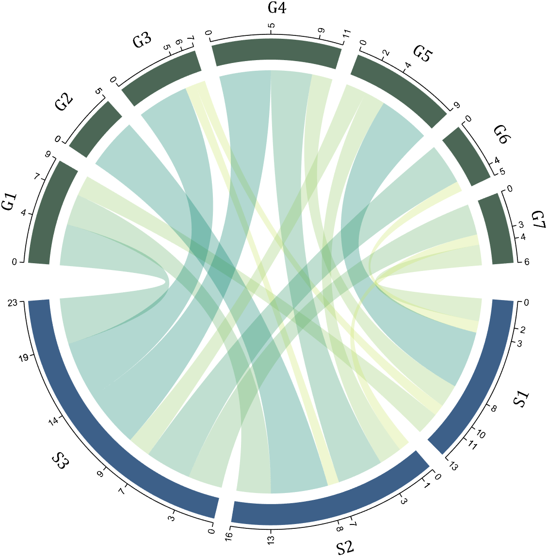
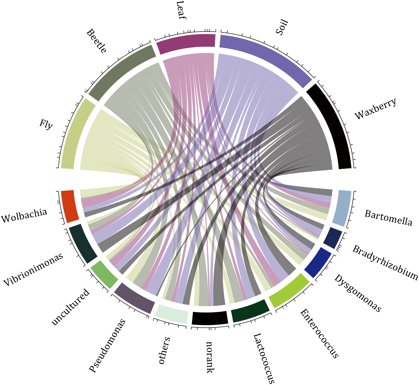
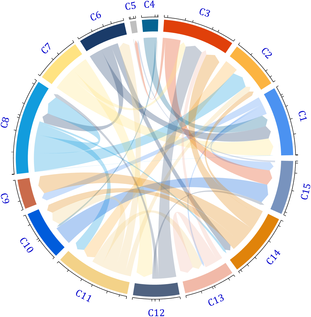
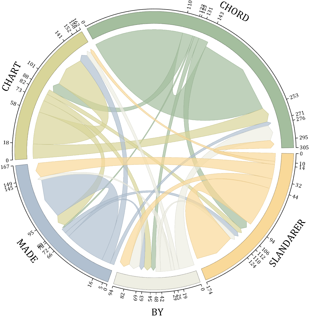
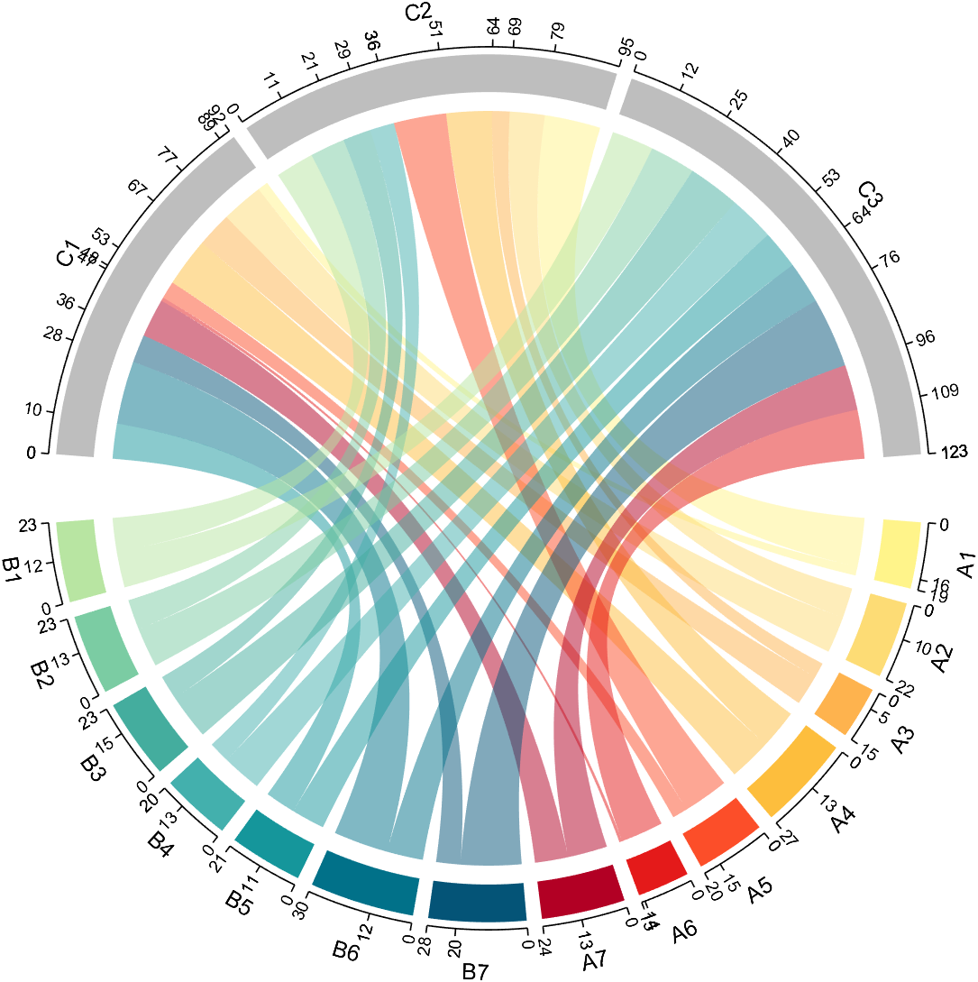
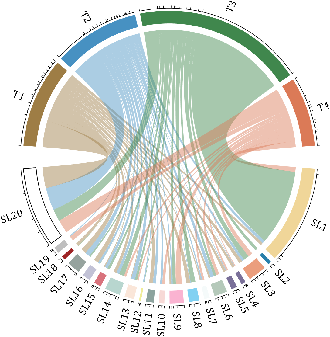
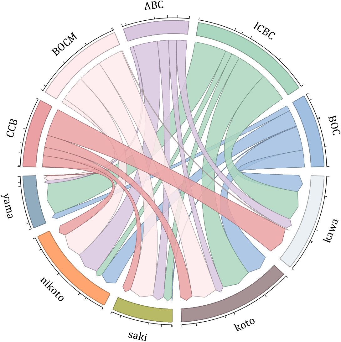
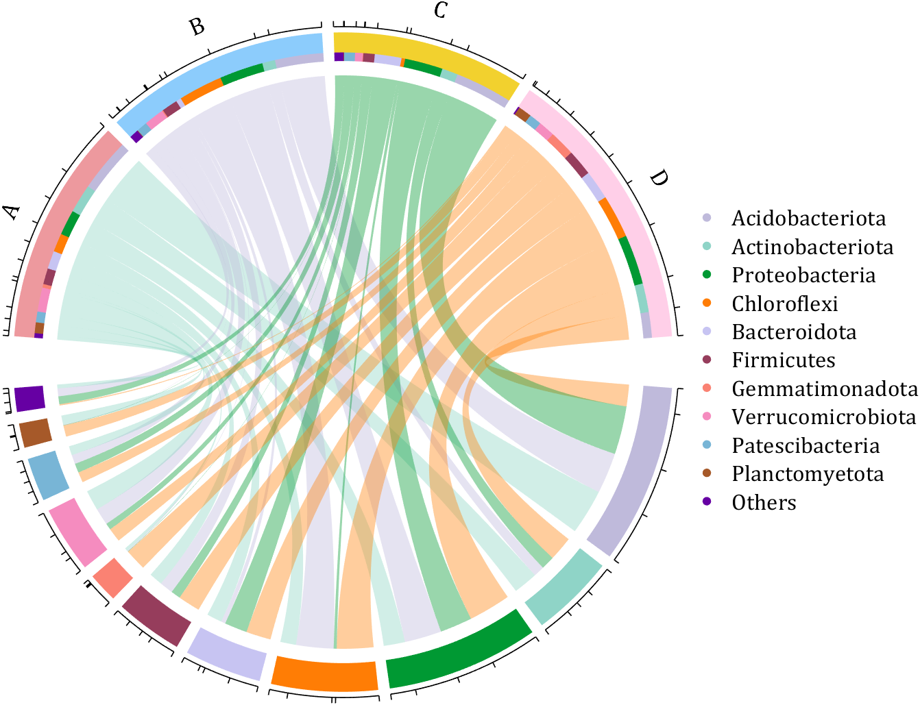
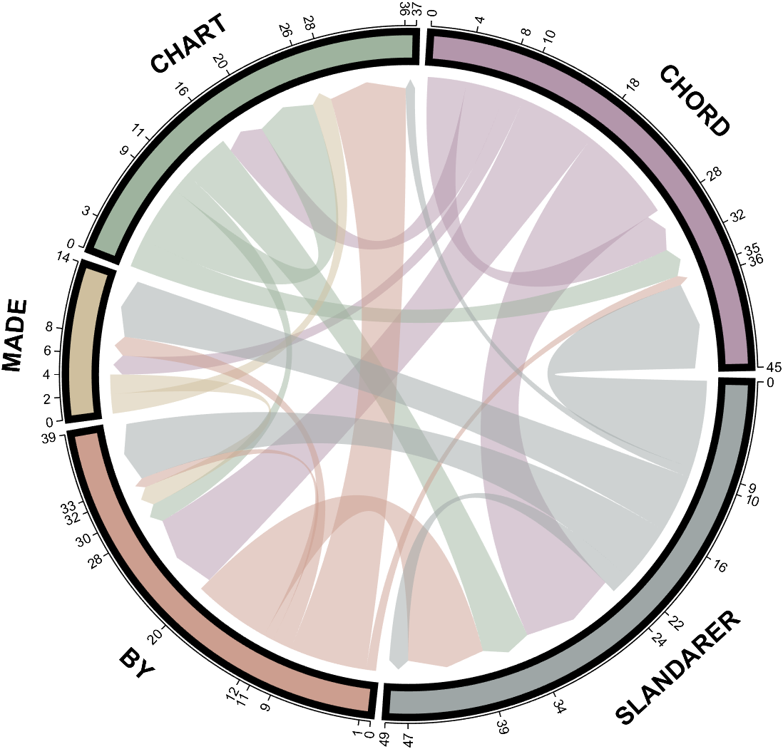
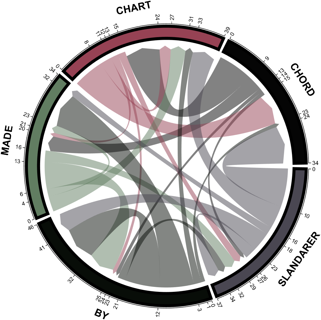
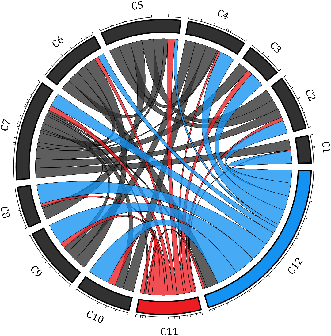
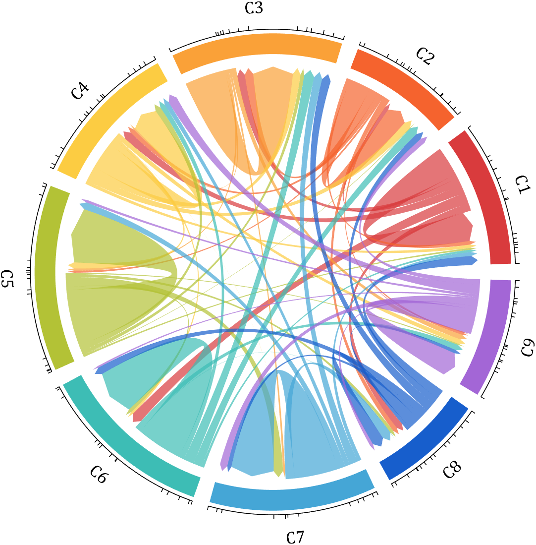
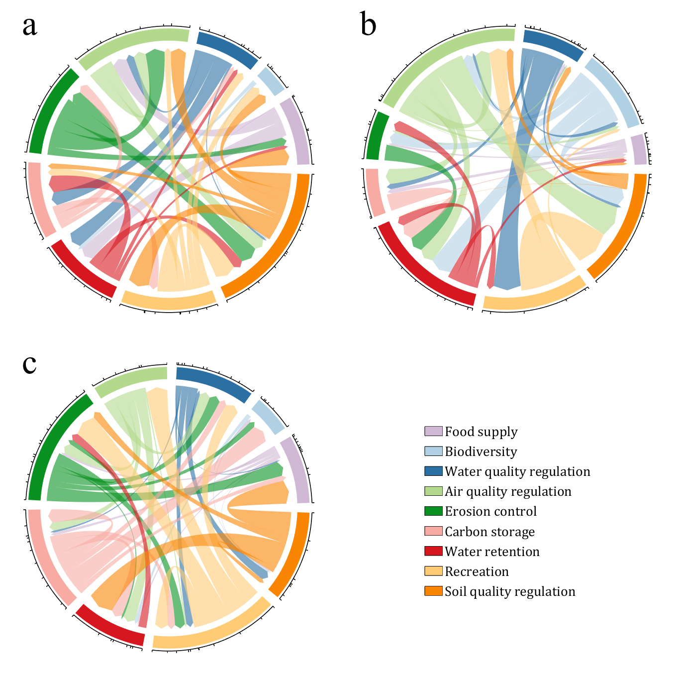
Chord diagrams are very common in Python and R, but there are no related functions in MATLAB before. It is not easy to draw chord diagrams of the same quality as R language, But I created a MATLAB tool that could almost do it.
The data requirement is a numerical matrix with all values greater than or equal to 0, or a table array, or a numerical matrix and cell array for names. First, give an example of a numerical matrix:
1.1 Numerical Matrix
dataMat=randi([0,5],[5,4]);
% 绘图(draw)
CC=chordChart(dataMat);
CC=CC.draw();
Since each object is not named, it will be automatically named Rn and Cn
RowName should be the same size as the rows of the matrix
ColName should be the same size as the columns of the matrix
For this example, if the value in the second row and third column is 1, it indicates that there is an energy flow from S2 to G3, and a chord with a width of 1 is needed between these two.
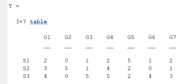
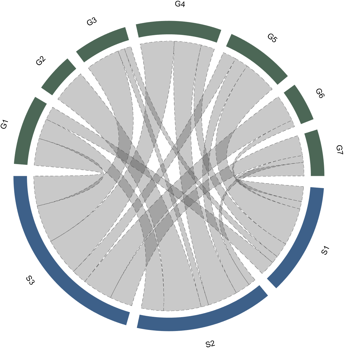
1.3 Table Array
A table array in the following format is required:
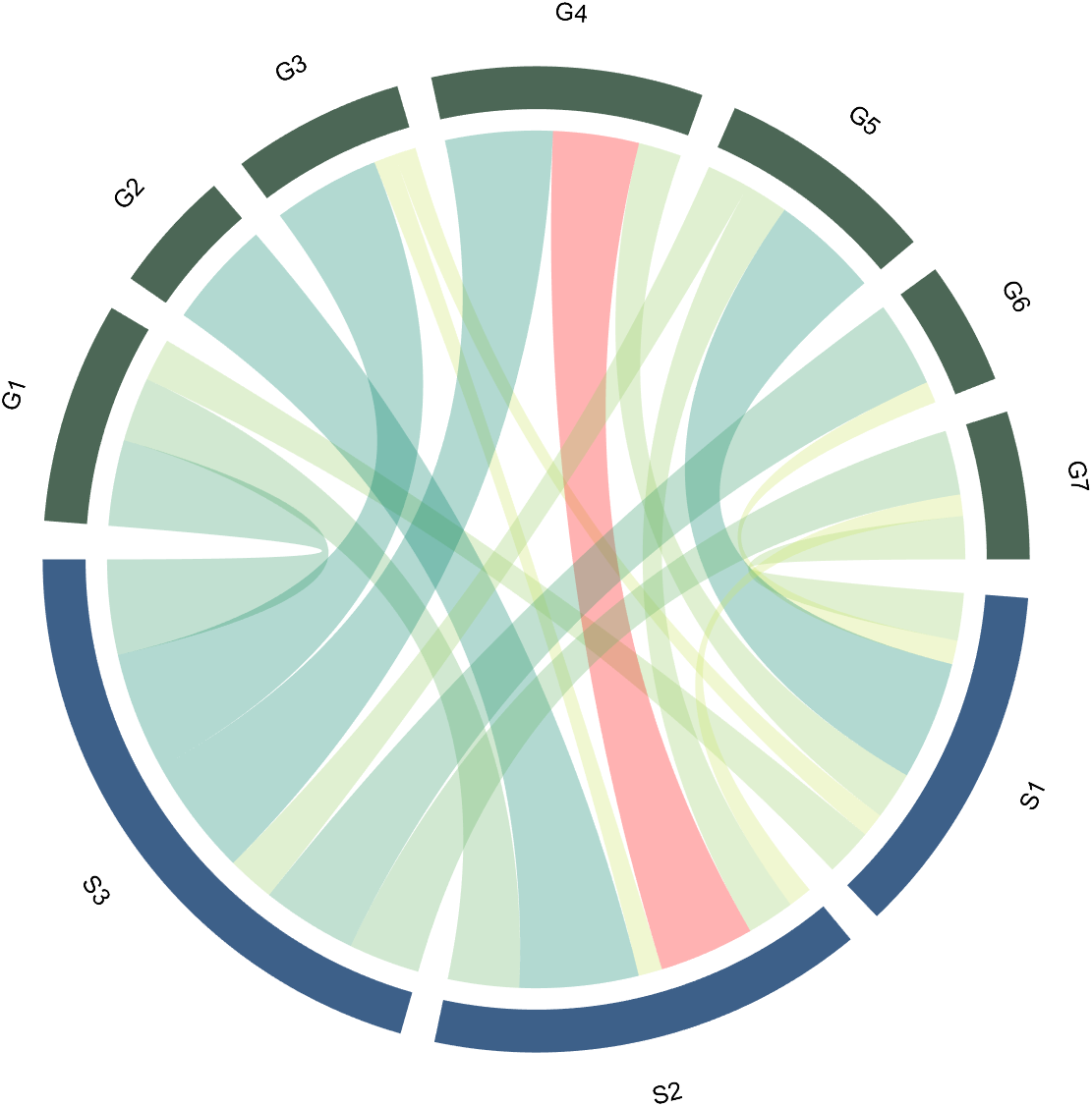
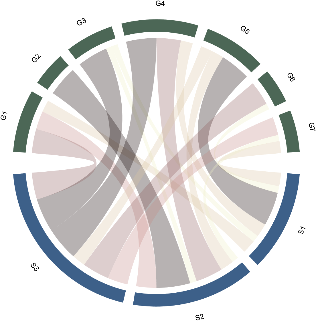
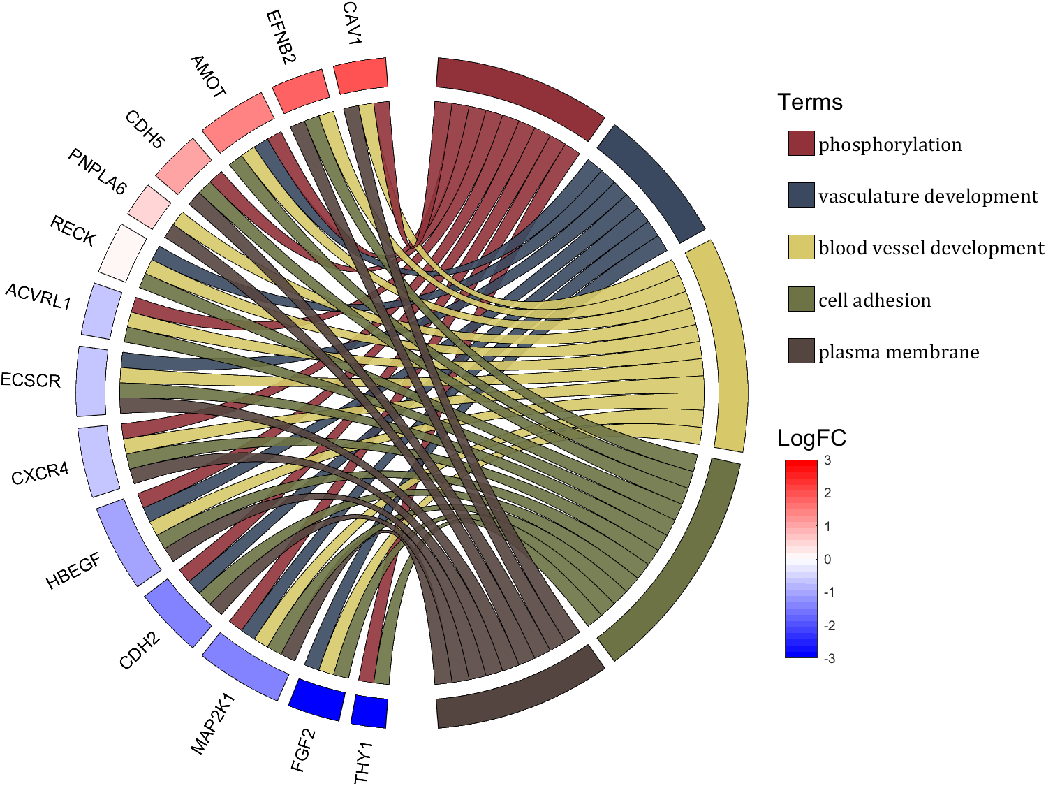
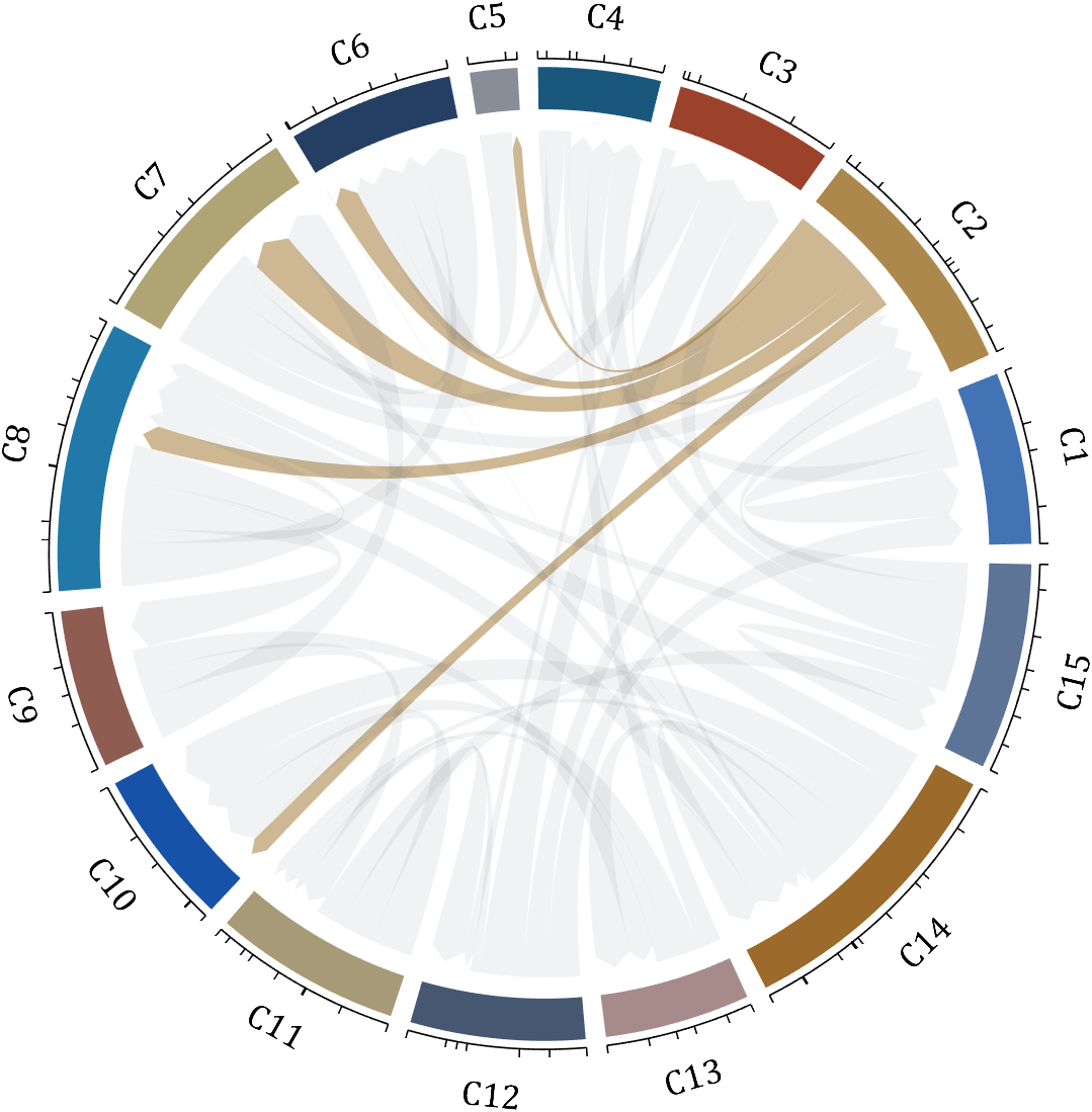
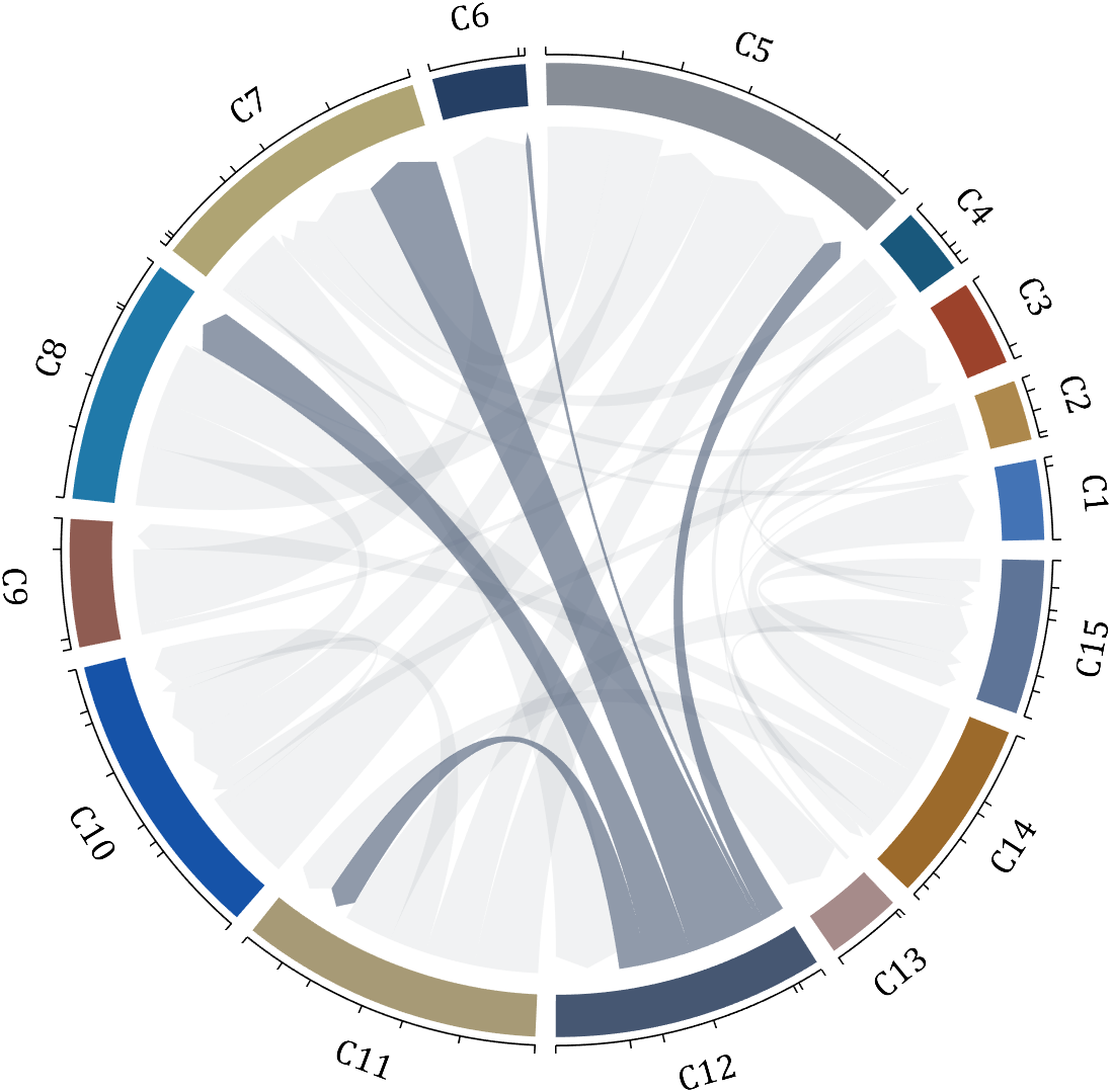
2 Decorate Chord
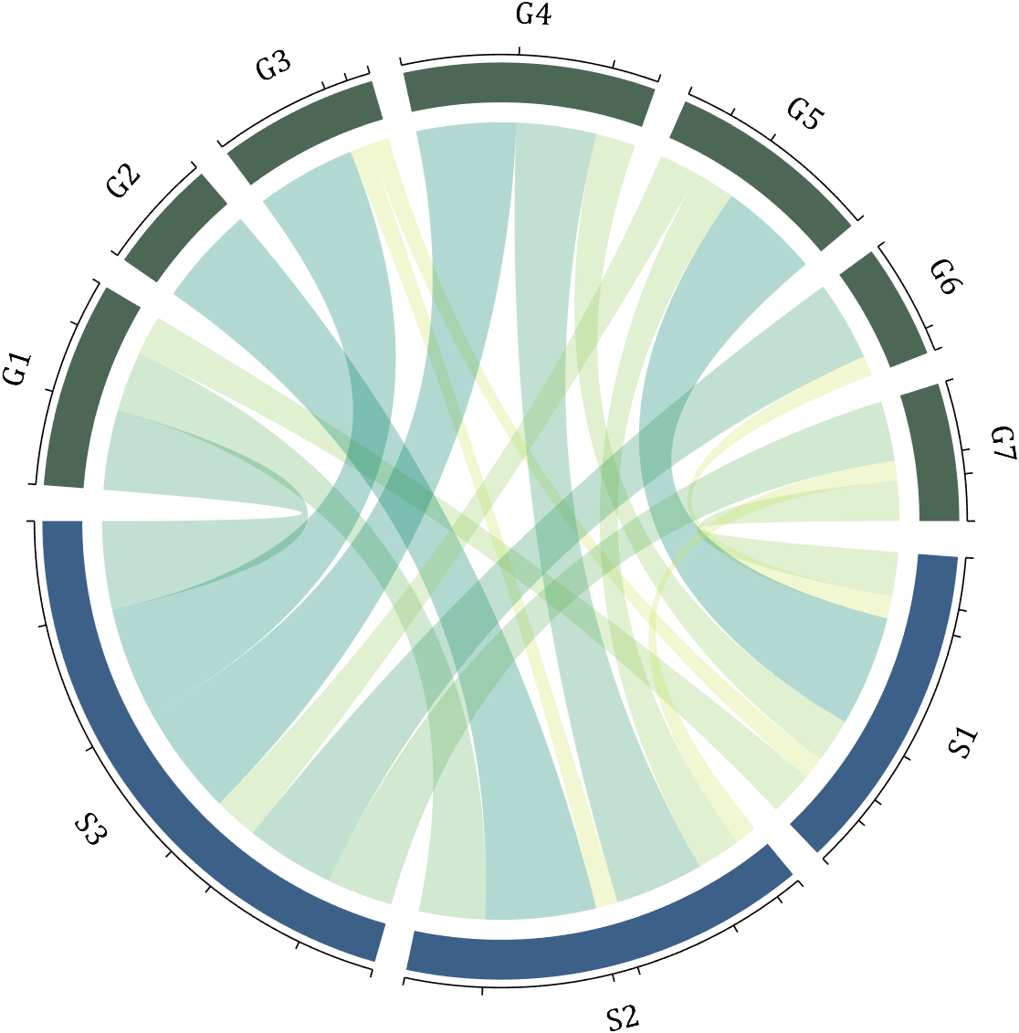
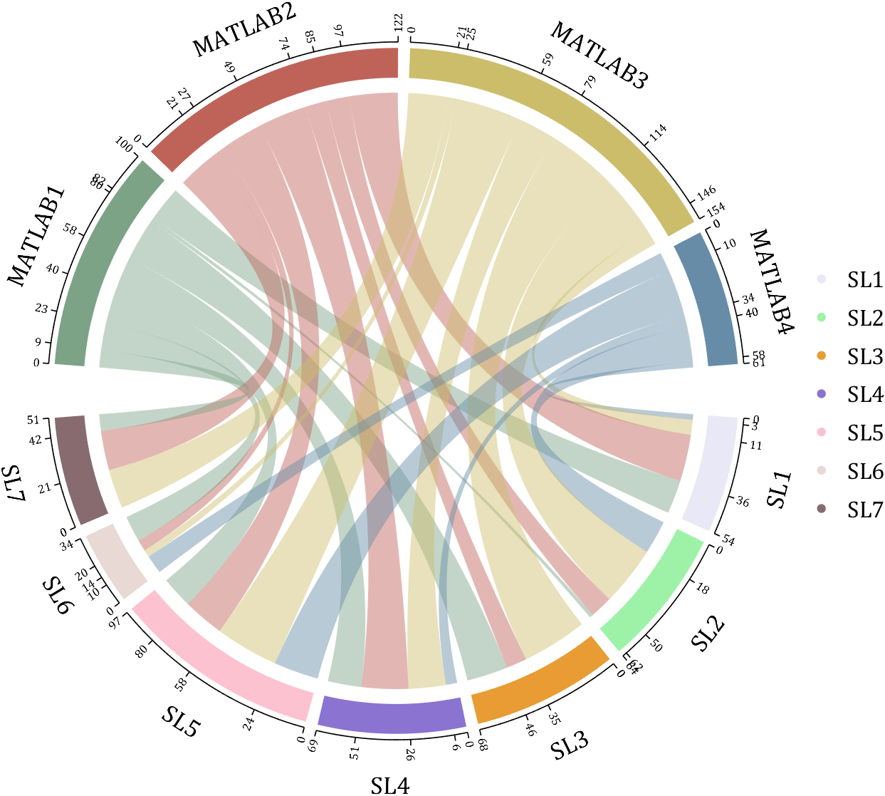
2.1 Batch modification of chords
Batch modification of chords can be done using the setChordProp function, and all properties of the Patch object can be modified. For example, modifying the color of the string, edge color, edge line sstyle, etc.:
The individual modification of chord can be done using the setChordMN function, where the values of m and n correspond exactly to the rows and columns of the original numerical matrix. For example, changing the color of the strings flowing from S2 to G4 to red:
CC.setChordMN(2,4,'FaceColor',[1,0,0])
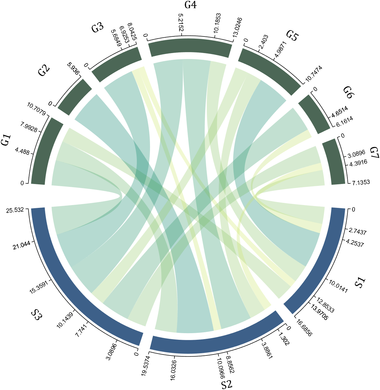
2.3 Color Mapping of Chords
Just use function colormap to do so:
% version 1.7.0更新
% 可使用colormap函数直接修改颜色
% Colors can be adjusted directly using the function colormap(demo4)
colormap(flipud(pink))
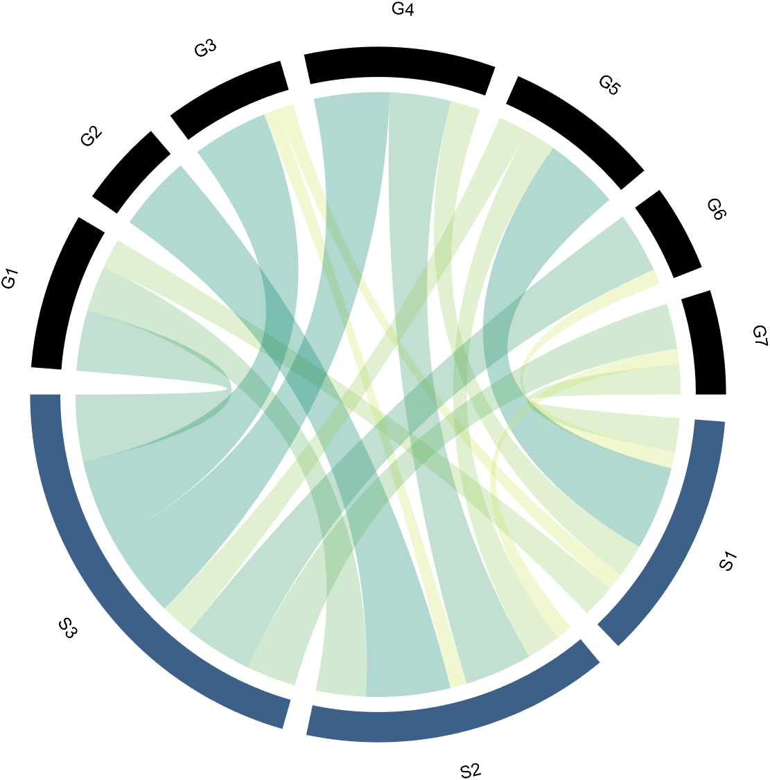
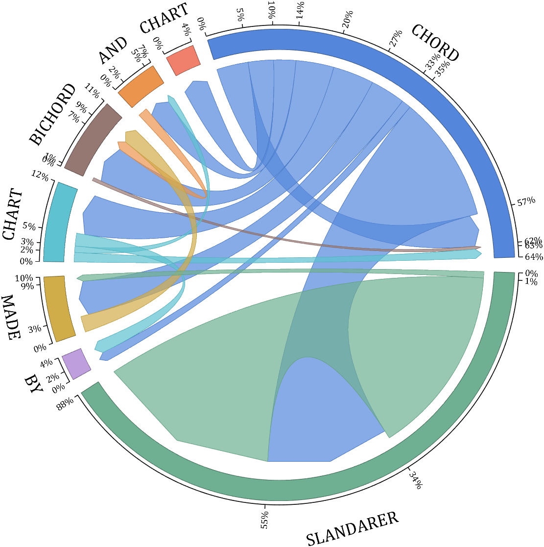
3 Arc Shaped Block Decoration
3.1 Batch Decoration of Arc-Shaped Blocks
use:
setSquareT_Prop
setSquareF_Prop
to modify the upper and lower blocks separately, and all attributes of the Patch object can be modified. For example, batch modify the upper blocks (change to black):
CC.setSquareT_Prop('FaceColor',[0,0,0])
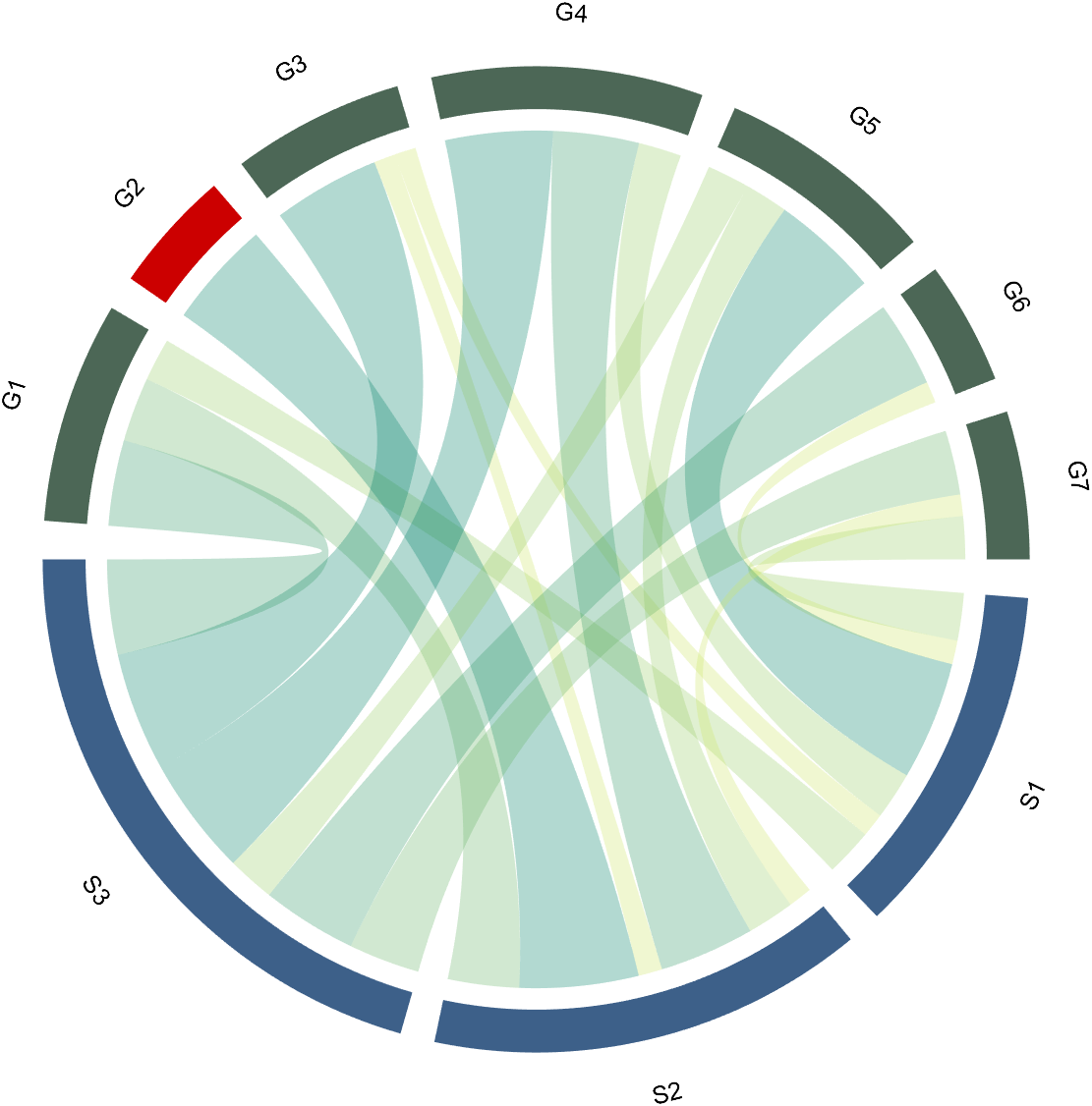
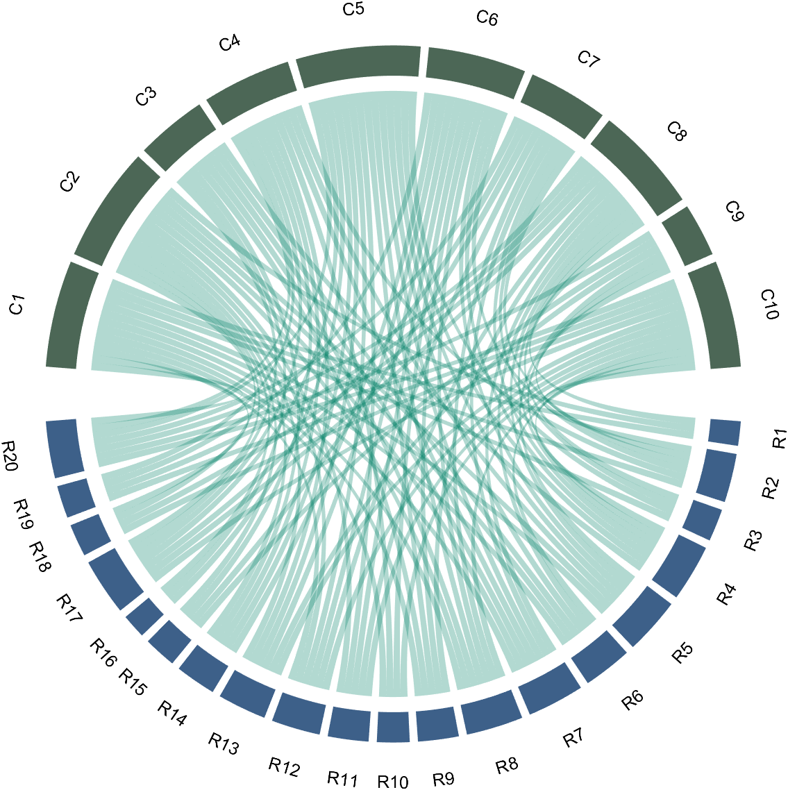
3.2 Arc-Shaped Blocks Individually Decoration
use:
setSquareT_N
setSquareF_N
to modify the upper and lower blocks separately. For example, modify the second block above separately (changed to red):
CC.setSquareT_N(2,'FaceColor',[.8,0,0])
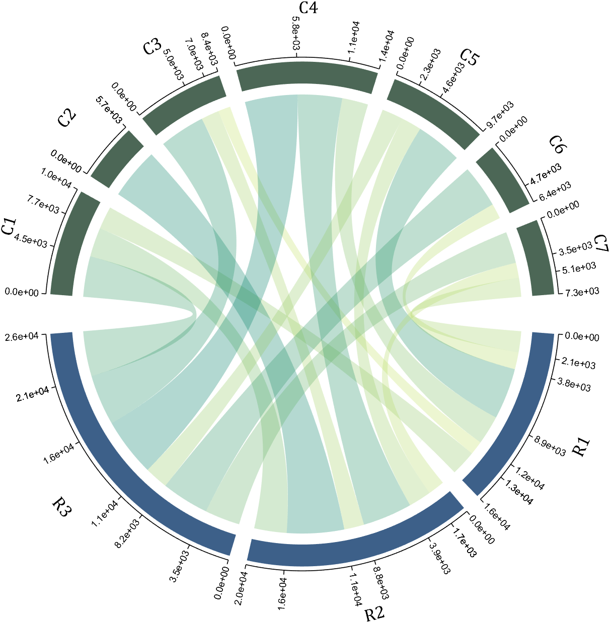
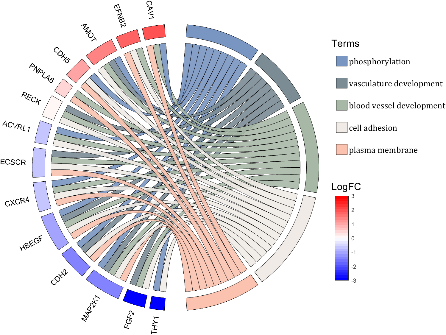
4 Font Adjustment
Use the setFont function to adjust the font, and all properties of the text object can be modified. For example, changing the font size, font, and color of the text:
A function handle is required to input numeric output strings. The format can be set through the setTickLabelFormat function, such as Scientific notation:
Most of my projects are the tension between what exists and what I must create to make the project work. The more I leverage what exists, the faster I can complete my project in a shorter amount of time. I often find out later in the process that a MATLAB function already exists and has existed for 10 releases. The faster that I discover built-in functions, the faster I can get to the new stuff that I have to invent.
I asked the AI Chat Playground why to use MATLAB's builtin functions and I got some interesting ideas. What are your thoughts?
AI Chat Playground:
Efficiency and Performance: MATLAB's built-in functions are highly optimized for performance. They are written in optimized and compiled languages like C or C++, which means they run faster than equivalent functions written directly in MATLAB language. When you use these functions, your code can execute more efficiently, which is especially beneficial for handling large datasets or complex mathematical computations.
Reliability and Stability: Built-in functions have been rigorously tested and debugged by the developers at MathWorks (the company behind MATLAB). They are less likely to contain errors compared to custom-written code, which means you can rely on them to produce accurate and consistent results.
Ease of Use: Built-in functions are designed to be user-friendly, with clear documentation and support materials available. This can make it easier to perform complex operations without needing a deep understanding of the underlying algorithms. It also reduces the amount of code you need to write and debug, saving time and reducing the potential for errors.
Compatibility: Built-in functions are updated alongside MATLAB itself, ensuring compatibility with new features and versions of the software. Using built-in functions can help ensure that your code continues to work correctly as MATLAB evolves.
Advanced Features: MATLAB’s built-in functions often include advanced features and options that are not readily available or would be difficult to implement on your own. For example, MATLAB’s mathematical functions can handle a wide range of special cases and data types, providing more flexibility than custom implementations.
Community and Support: Using built-in functions means you're working with standard tools recognized by the MATLAB community. This can make it easier to get help from other users or from MathWorks support, as more people will be familiar with the functionality and potential issues of these functions.


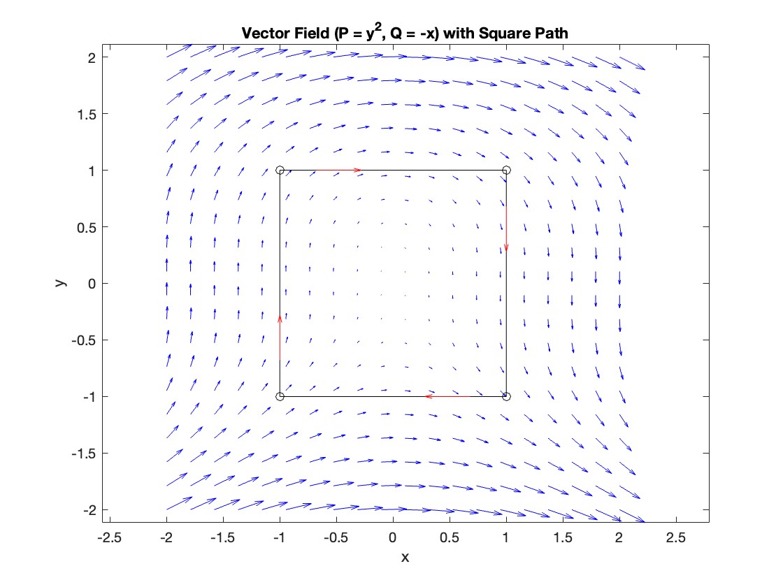
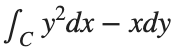 , where C is the boundary of the square
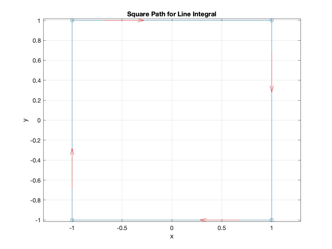
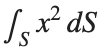 over the sphere
  are symmetric, you can exploit these symmetries to simplify the calculation.