結果:

0 - 3 / 3

General

Athanasios Paraskevopoulos
最後のアクティビティ: 2024 年 7 月 23 日

Gabriel's Horn

Gabriel's horn is a shape with the paradoxical property that it has infinite surface area, but a finite volume.

Gabriel’s horn is formed by taking the graph of

with the domain

and rotating it in three dimensions about the

axis.

There is a standard formula for calculating the volume of this shape, for a general function

.Wwe will just state that the volume of the

solid between a and b is:

The surface area of the solid is given by:

One other thing we need to consider is that we are trying to find the value of these integrals between 1 and ∞. An integral with a limit of infinity is called an improper integral and we can't evaluate it simply by plugging the value infinity into the normal equation for a definite integral. Instead, we must first calculate the definite integral up to some finite limit b and then calculate the limit of the result as b tends to ∞:

Volume

We can calculate the horn's volume using the volume integral above, so

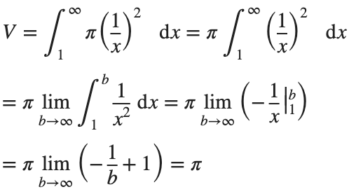
The total volume of this infinitely long trumpet isπ.

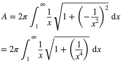
Surface Area

To determine the surface area, we first need the function’s derivative:

Now plug it into the surface area formula and we have:

This is an improper integral and it's hard to evaluate, but since in our interval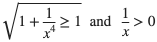

So, we have :

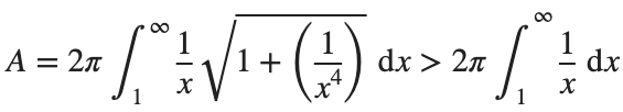
Now,we evaluate this last integral

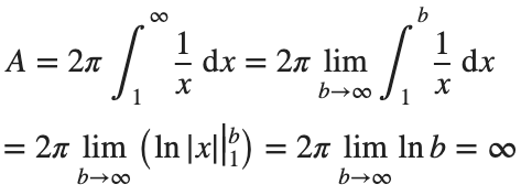
So the surface are is infinite.

% Define the function for Gabriel's Horn

gabriels_horn = @(x) 1 ./ x;

% Create a range of x values

x = linspace(1, 40, 4000); % Increase the number of points for better accuracy

y = gabriels_horn(x);

% Create the meshgrid

theta = linspace(0, 2 * pi, 6000); % Increase theta points for a smoother surface

[X, T] = meshgrid(x, theta);

Y = gabriels_horn(X) .* cos(T);

Z = gabriels_horn(X) .* sin(T);

% Plot the surface of Gabriel's Horn

figure('Position', [200, 100, 1200, 900]);

surf(X, Y, Z, 'EdgeColor', 'none', 'FaceAlpha', 0.9);

hold on;

% Plot the central axis

plot3(x, zeros(size(x)), zeros(size(x)), 'r', 'LineWidth', 2);

% Set labels

xlabel('x');

ylabel('y');

zlabel('z');

% Adjust colormap and axis properties

colormap('gray');

shading interp; % Smooth shading

% Adjust the view

view(3);

axis tight;

grid on;

% Add formulas as text annotations

dim1 = [0.4 0.7 0.3 0.2];

annotation('textbox',dim1,'String',{'$$V = \pi \int_{1}^{a} \left( \frac{1}{x} \right)^2 dx = \pi \left( 1 - \frac{1}{a} \right)$$', ...

'', ... % Add an empty line for larger gap

'$$\lim_{a \to \infty} V = \lim_{a \to \infty} \pi \left( 1 - \frac{1}{a} \right) = \pi$$'}, ...

'Interpreter','latex','FontSize',12, 'EdgeColor','none', 'FitBoxToText', 'on');

dim2 = [0.4 0.5 0.3 0.2];

annotation('textbox',dim2,'String',{'$$A = 2\pi \int_{1}^{a} \frac{1}{x} \sqrt{1 + \left( -\frac{1}{x^2} \right)^2} dx > 2\pi \int_{1}^{a} \frac{dx}{x} = 2\pi \ln(a)$$', ...

'', ... % Add an empty line for larger gap

'$$\lim_{a \to \infty} A \geq \lim_{a \to \infty} 2\pi \ln(a) = \infty$$'}, ...

'Interpreter','latex','FontSize',12, 'EdgeColor','none', 'FitBoxToText', 'on');

% Add Gabriel's Horn label

dim3 = [0.3 0.9 0.3 0.1];

annotation('textbox',dim3,'String','Gabriel''s Horn', ...

'Interpreter','latex','FontSize',14, 'EdgeColor','none', 'HorizontalAlignment', 'center');

hold off

daspect([3.5 1 1]) % daspect([x y z])

view(-27, 15)

lightangle(-50,0)

lighting('gouraud')

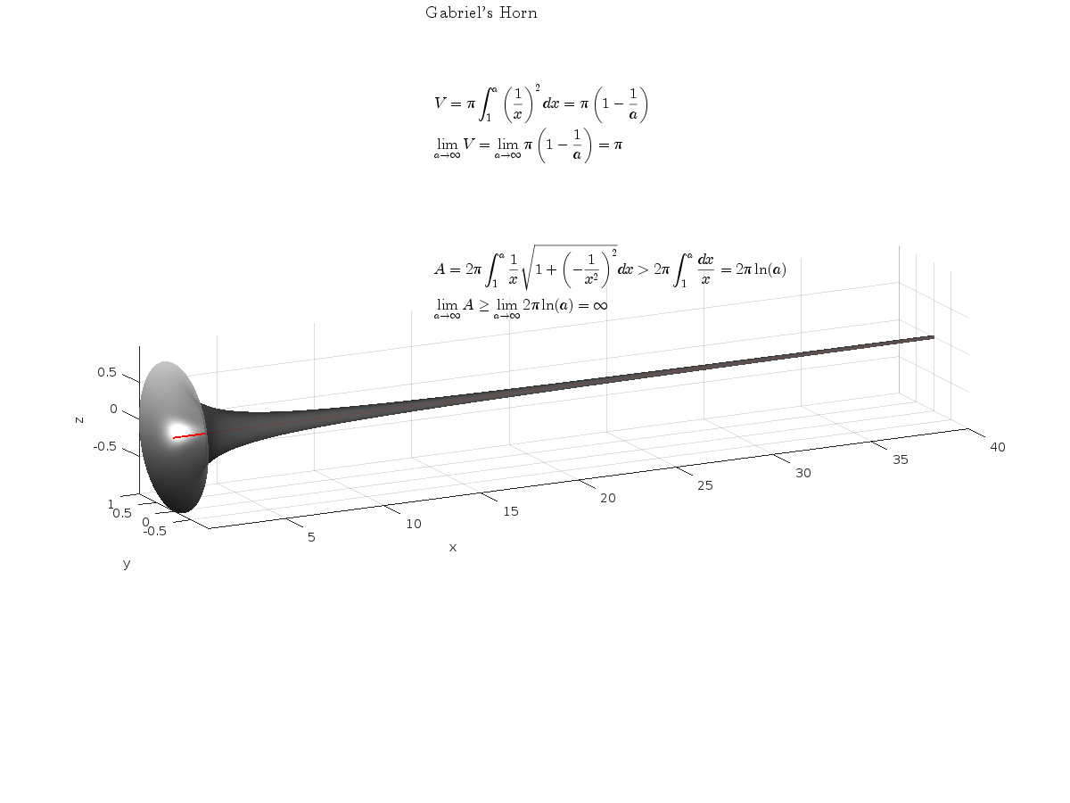
The properties of this figure were first studied by Italian physicist and mathematician Evangelista Torricelli in the 17th century.

Acknowledgment

I would like to express my sincere gratitude to all those who have supported and inspired me throughout this project.

First and foremost, I would like to thank the mathematician and my esteemed colleague, Stavros Tsalapatis, for inspiring me with the fascinating subject of Gabriel's Horn.

I am also deeply thankful to Mr. @Star Strider for his invaluable assistance in completing the final code.

References:

Tips & Tricks

Athanasios Paraskevopoulos
最後のアクティビティ: 2024 年 3 月 31 日

Analysis and Visualization of Line Integral and Green's Theorem on a Square Path

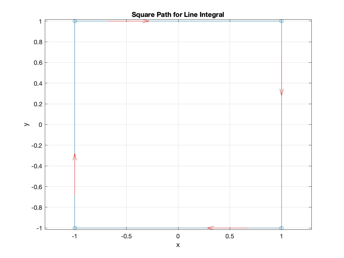
The line integral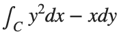

, where C is the boundary of the square

oriented counterclockwise, can be evaluated in two ways:

Using the definition of the line integral:

% Initialize the integral sum
integral_sum = 0;
% Segment C1: x = -1, y goes from -1 to 1
y = linspace(-1, 1);
x = -1 * ones(size(y));
dy = diff(y);
integral_sum = integral_sum + sum(-x(1:end-1) .* dy);
% Segment C2: y = 1, x goes from -1 to 1
x = linspace(-1, 1);
y = ones(size(x));
dx = diff(x);
integral_sum = integral_sum + sum(y(1:end-1).^2 .* dx);
% Segment C3: x = 1, y goes from 1 to -1
y = linspace(1, -1);
x = ones(size(y));
dy = diff(y);
integral_sum = integral_sum + sum(-x(1:end-1) .* dy);
% Segment C4: y = -1, x goes from 1 to -1
x = linspace(1, -1);
y = -1 * ones(size(x));
dx = diff(x);
integral_sum = integral_sum + sum(y(1:end-1).^2 .* dx);
disp(['Direct Method Integral: ', num2str(integral_sum)]);

Plotting the square path

% Define the square's vertices
vertices = [-1 -1; -1 1; 1 1; 1 -1; -1 -1];
% Plot the square
figure;
plot(vertices(:,1), vertices(:,2), '-o');
title('Square Path for Line Integral');
xlabel('x');
ylabel('y');
grid on;
axis equal;
% Add arrows to indicate the path direction (counterclockwise)
hold on;
for i = 1:size(vertices,1)-1
    % Calculate direction
    dx = vertices(i+1,1) - vertices(i,1);
    dy = vertices(i+1,2) - vertices(i,2);
    % Reduce the length of the arrow for better visibility
    scale = 0.2;
    dx = scale * dx;
    dy = scale * dy;
    % Calculate the start point of the arrow
    startx = vertices(i,1) + (1 - scale) * dx;
    starty = vertices(i,2) + (1 - scale) * dy;
    % Plot the arrow
    quiver(startx, starty, dx, dy, 'MaxHeadSize', 0.5, 'Color', 'r', 'AutoScale', 'off');
end
hold off;

Apply Green's Theorem for the line integral

% Define the partial derivatives of P and Q
f = @(x, y) -1 - 2*y;  % derivative of -x with respect to x is -1, and derivative of y^2 with respect to y is 2y
% Compute the double integral over the square [-1,1]x[-1,1]
integral_value = integral2(f, -1, 1, 1, -1);
disp(['Green''s Theorem Integral: ', num2str(integral_value)]);

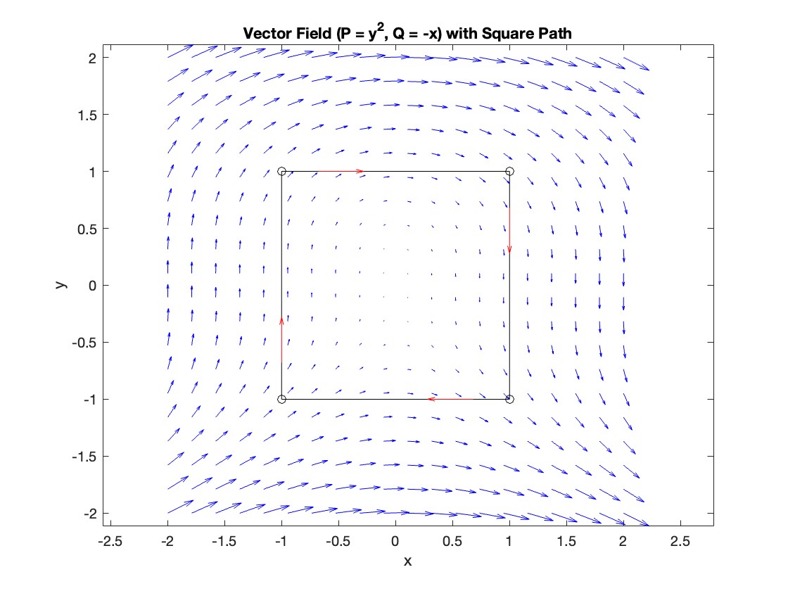
Plotting the vector field related to Green’s theorem

% Define the grid for the vector field
[x, y] = meshgrid(linspace(-2, 2, 20), linspace(-2 ,2, 20));
% Define the vector field components
P = y.^2;  % y^2 component
Q = -x;    % -x component
% Plot the vector field
figure;
quiver(x, y, P, Q, 'b');
hold on;  % Hold on to plot the square on the same figure
% Define the square's vertices
vertices = [-1 -1; -1 1; 1 1; 1 -1; -1 -1];
% Plot the square path
plot(vertices(:,1), vertices(:,2), '-o', 'Color', 'k');  % 'k' for black color
title('Vector Field (P = y^2, Q = -x) with Square Path');
xlabel('x');
ylabel('y');
axis equal;
% Add arrows to indicate the path direction (counterclockwise)
for i = 1:size(vertices,1)-1
    % Calculate direction
    dx = vertices(i+1,1) - vertices(i,1);
    dy = vertices(i+1,2) - vertices(i,2);
    % Reduce the length of the arrow for better visibility
    scale = 0.2;
    dx = scale * dx;
    dy = scale * dy;
    % Calculate the start point of the arrow
    startx = vertices(i,1) + (1 - scale) * dx;
    starty = vertices(i,2) + (1 - scale) * dy;
    % Plot the arrow
    quiver(startx, starty, dx, dy, 'MaxHeadSize', 0.5, 'Color', 'r', 'AutoScale', 'off');
end
hold off;

Tips & Tricks

Athanasios Paraskevopoulos
最後のアクティビティ: 2024 年 3 月 29 日

Computing a Surface Integral on a Sphere Using MATLAB

To solve a surface integral for example the

over the sphere

easily in MATLAB, you can leverage the symbolic toolbox for a direct and clear solution. Here is a tip to simplify the process:

Use Symbolic Variables and Functions: Define your variables symbolically, including the parameters of your spherical coordinates θ and ϕ and the radius r . This allows MATLAB to handle the expressions symbolically, making it easier to manipulate and integrate them.
Express in Spherical Coordinates Directly: Since you already know the sphere's equation and the relationship in spherical coordinates, define x, y, and z in terms of r , θ and ϕ directly.
Perform Symbolic Integration: Use MATLAB's `int` function to integrate symbolically. Since the sphere and the function are symmetric, you can exploit these symmetries to simplify the calculation.

Here’s how you can apply this tip in MATLAB code:

% Include the symbolic math toolbox
syms theta phi
% Define the limits for theta and phi
theta_limits = [0, pi];
phi_limits = [0, 2*pi];
% Define the integrand function symbolically
integrand = 16 * sin(theta)^3 * cos(phi)^2;
% Perform the symbolic integral for the surface integral
surface_integral = int(int(integrand, theta, theta_limits(1), theta_limits(2)), phi, phi_limits(1), phi_limits(2));
% Display the result of the surface integral symbolically
disp(['The surface integral of x^2 over the sphere is ', char(surface_integral)]);
% Number of points for plotting
num_points = 100;
% Define theta and phi for the sphere's surface
[theta_mesh, phi_mesh] = meshgrid(linspace(double(theta_limits(1)), double(theta_limits(2)), num_points), ...
                                  linspace(double(phi_limits(1)), double(phi_limits(2)), num_points));
% Spherical to Cartesian conversion for plotting
r = 2; % radius of the sphere
x = r * sin(theta_mesh) .* cos(phi_mesh);
y = r * sin(theta_mesh) .* sin(phi_mesh);
z = r * cos(theta_mesh);
% Plot the sphere
figure;
surf(x, y, z, 'FaceColor', 'interp', 'EdgeColor', 'none');
colormap('jet'); % Color scheme
shading interp; % Smooth shading
camlight headlight; % Add headlight-type lighting
lighting gouraud; % Use Gouraud shading for smooth color transitions
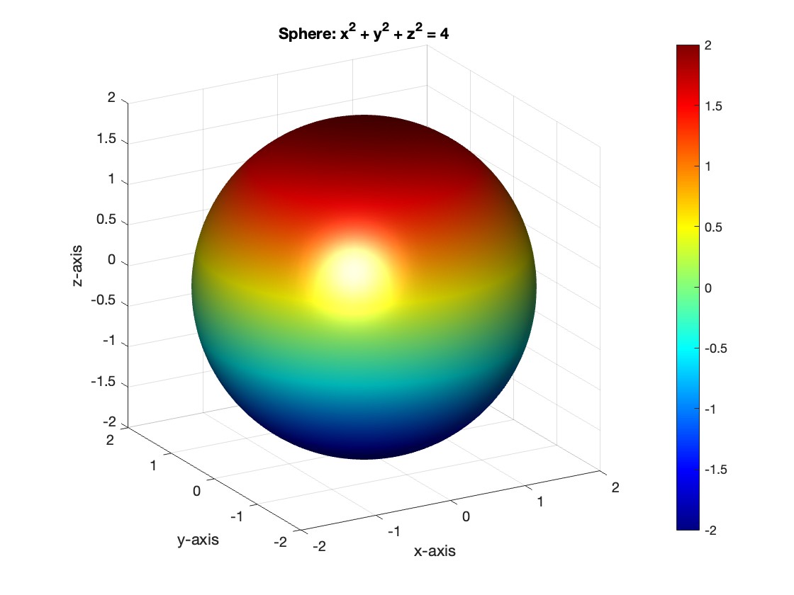
title('Sphere: x^2 + y^2 + z^2 = 4');
xlabel('x-axis');
ylabel('y-axis');
zlabel('z-axis');
colorbar; % Add color bar to indicate height values
axis square; % Maintain aspect ratio to be square
view([-30, 20]); % Set a nice viewing angle

0 - 3 / 3