結果:
- Introduction to ODEs: Basic concepts, definitions, and initial differential equations.
- Methods of Solution:
- Separable equations
- First-order linear equations
- Exact equations
- Transcendental functions
- Applications of ODEs: Practical examples and applications in various scientific fields.
- Systems of ODEs: Analysis and solutions of systems of differential equations.
- Series and Numerical Methods: Use of series and numerical methods for solving ODEs.

 $ is the unknown displacement of the oscillator occupying the n-th position of the lattice, and
 and
and  , that is,
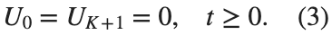
 for the one-dimensional discrete Laplacian
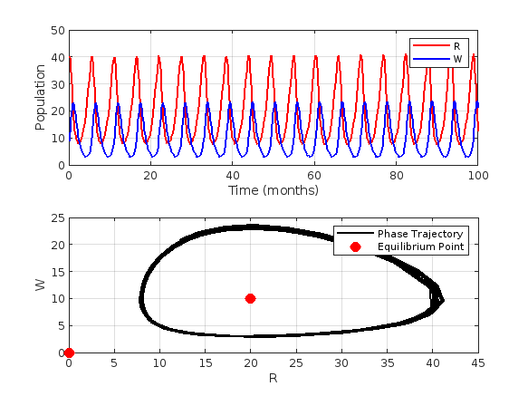
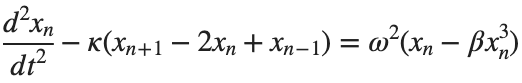
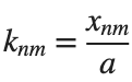
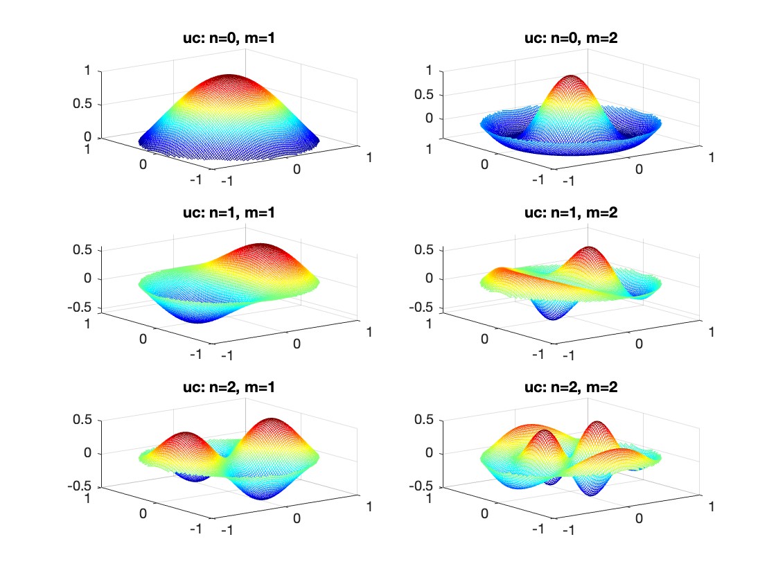
 . We consider spatially extended initial conditions of the form:
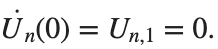
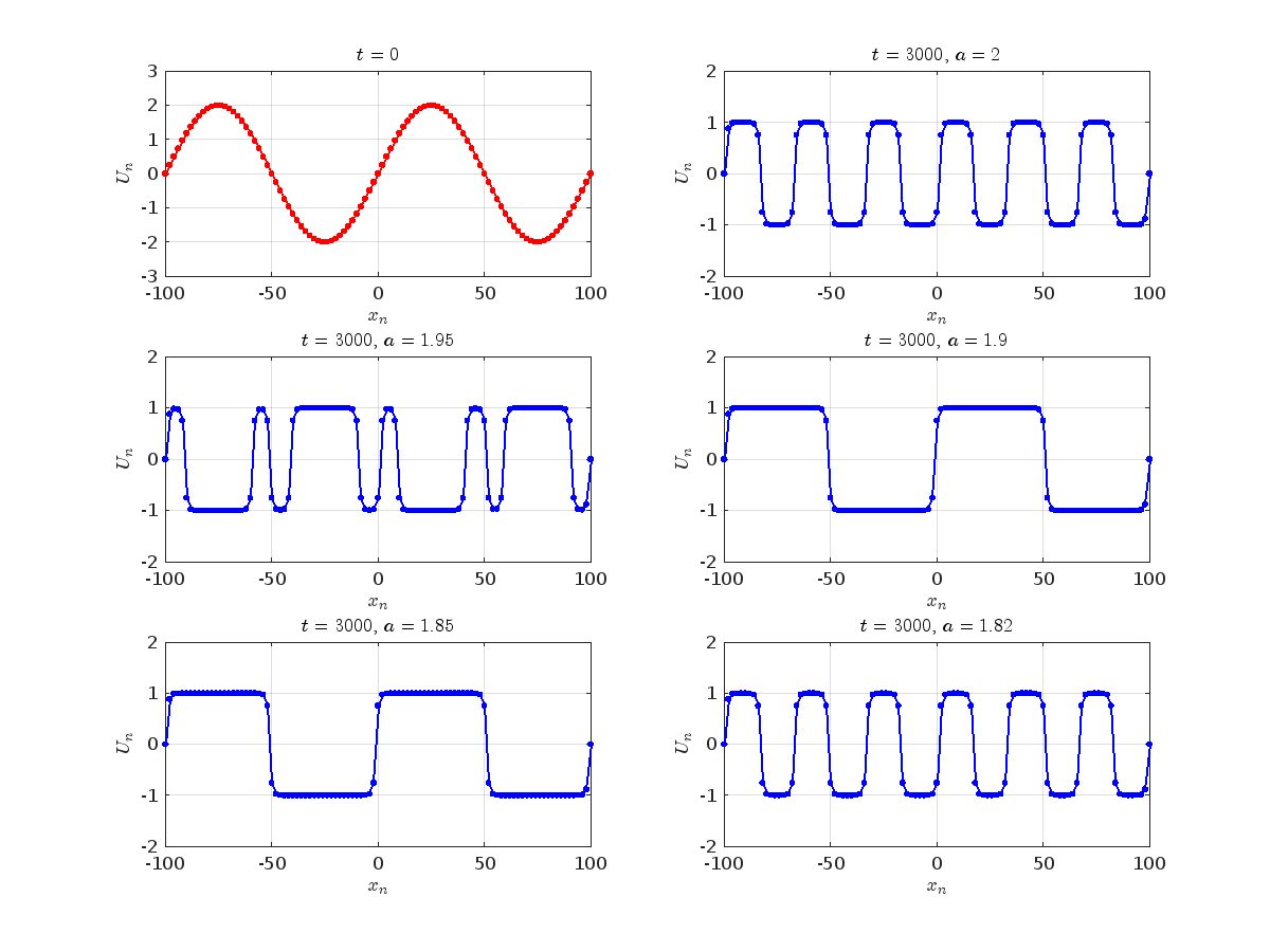
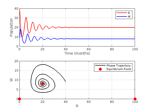
 where the dynamics appear in the first image of the third row, we observe convergence to a non-linear equilibrium point of branch
  respectively, converges to a non-linear equilibrium point of branch
  and energy
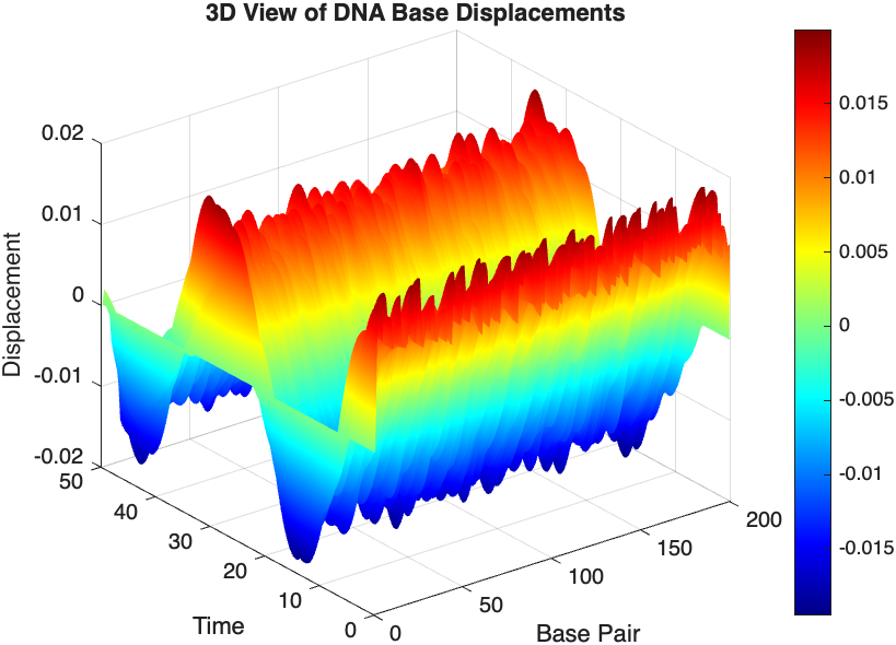
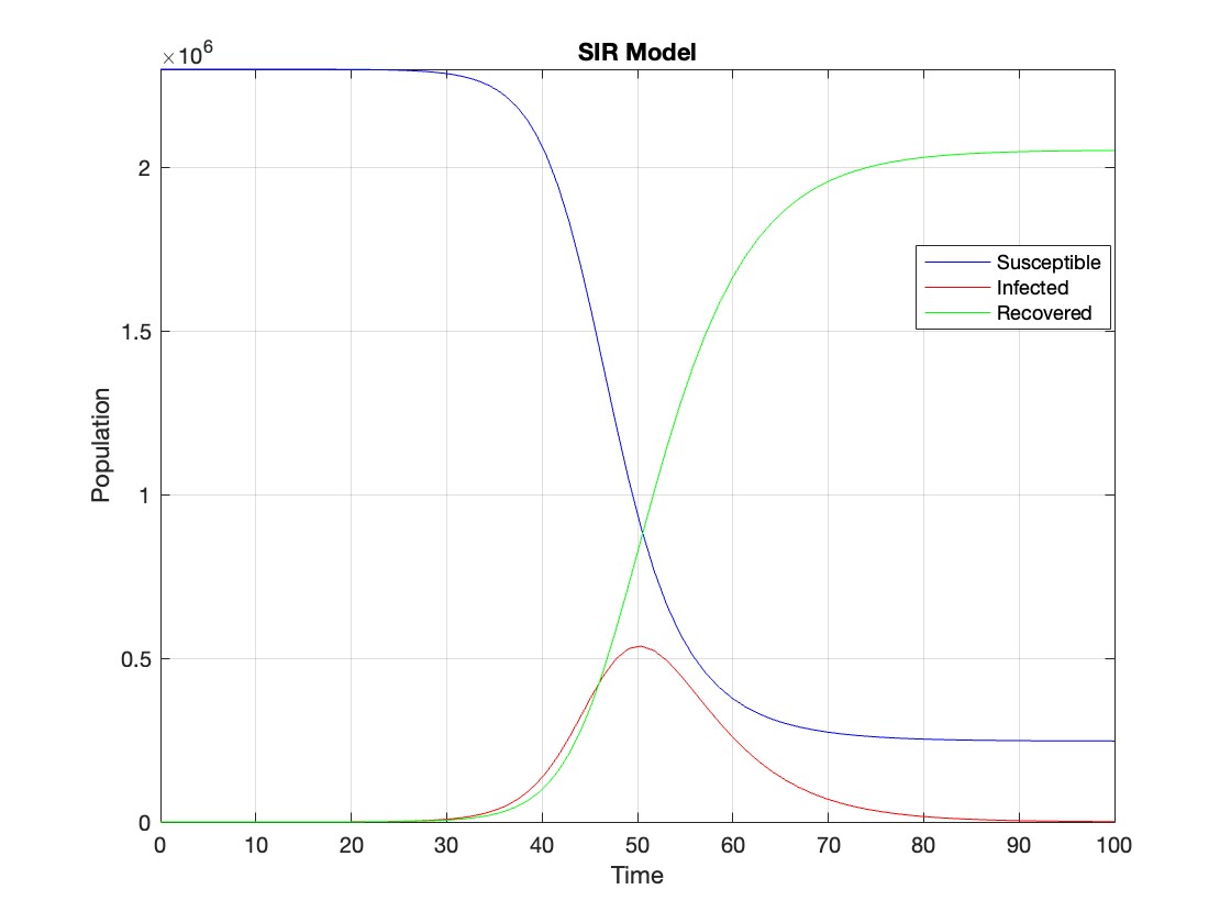
- Position: Random initial perturbations between 0.01 and 0.02 to simulate the thermal fluctuations at the start.
- Velocity: All bases start from rest, assuming no initial movement except for the thermal perturbations.
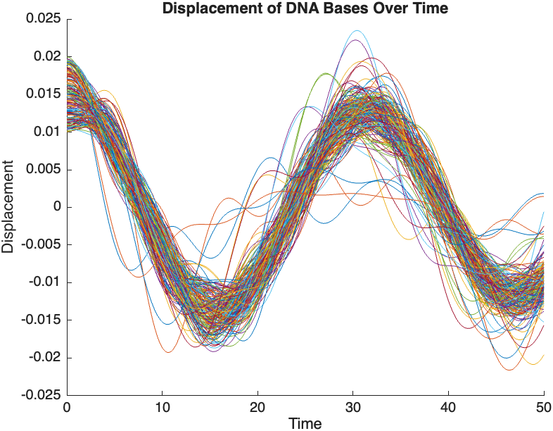
- Wave Propagation: The initial perturbations lead to wave-like dynamics along the segment, with visible propagation and reflection at the boundaries.
- Damping Effects: The inclusion of damping leads to a gradual reduction in the amplitude of the oscillations, indicating energy dissipation over time.
- Nonlinear Behavior: The nonlinear term influences the response, potentially stabilizing the system against large displacements or leading to complex dynamic patterns.
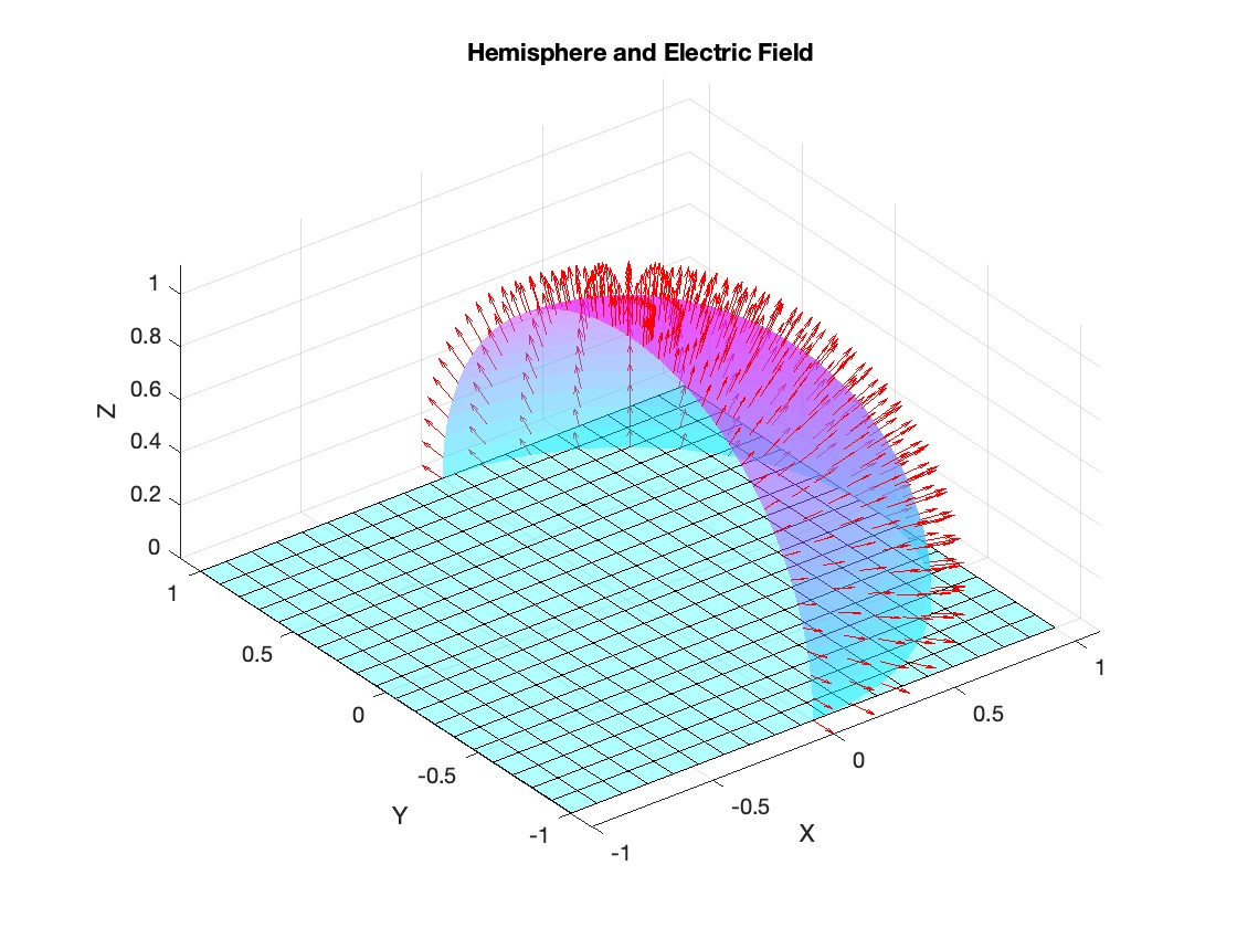
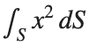 over the sphere
 - Use Symbolic Variables and Functions: Define your variables symbolically, including the parameters of your spherical coordinates θ and ϕ and the radius r . This allows MATLAB to handle the expressions symbolically, making it easier to manipulate and integrate them.
- Express in Spherical Coordinates Directly: Since you already know the sphere's equation and the relationship in spherical coordinates, define x, y, and z in terms of r , θ and ϕ directly.
- Perform Symbolic Integration: Use MATLAB's `int` function to integrate symbolically. Since the sphere and the function
 are symmetric, you can exploit these symmetries to simplify the calculation.
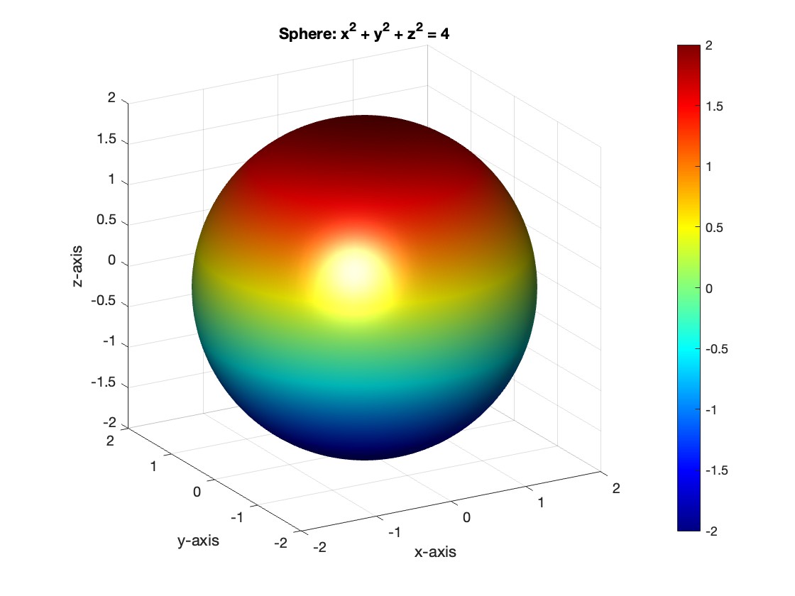
 , is zero, meaning the motion of the system does not change over time. This leads to a static differential equation:

The Symbolic Math Toolbox includes functions for solving, visualizing, and manipulating symbolic math equations. In combination with MATLAB’s Live Editor, it provides an easy, intuitive, and complete environment to interactively learn and teach algebra, calculus, and ordinary differential equations.
Starting with MATLAB R2021a, you can represent matrices and vectors in compact matrix notation with a new symbolic matrix variable data type. This enables a concise typeset display and show mathematical formulas with more clarity. Using them, you can show matrix- and vector-based expressions the way they are displayed in textbooks.
Contrast the visual difference between matrices of symbolic scalar variables and the new symbolic matrix variables:
The syms and symmatrix functions create symbolic matrix variables. To convert a symbolic matrix variable to an array of symbolic scalar variables, use symmatrix2sym. For an example, see Create Symbolic Matrix Variables.