メインコンテンツ
結果:
The study of the dynamics of the discrete Klein - Gordon equation (DKG) with friction is given by the equation :

above equation, W describes the potential function :
The objective of this simulation is to model the dynamics of a segment of DNA under thermal fluctuations with fixed boundaries using a modified discrete Klein-Gordon equation. The model incorporates elasticity, nonlinearity, and damping to provide insights into the mechanical behavior of DNA under various conditions.
% Parameters
numBases = 200; % Number of base pairs, representing a segment of DNA
kappa = 0.1; % Elasticity constant
omegaD = 0.2; % Frequency term
beta = 0.05; % Nonlinearity coefficient
delta = 0.01; % Damping coefficient
- Position: Random initial perturbations between 0.01 and 0.02 to simulate the thermal fluctuations at the start.
- Velocity: All bases start from rest, assuming no initial movement except for the thermal perturbations.
% Random initial perturbations to simulate thermal fluctuations
initialPositions = 0.01 + (0.02-0.01).*rand(numBases,1);
initialVelocities = zeros(numBases,1); % Assuming initial rest state
The simulation uses fixed ends to model the DNA segment being anchored at both ends, which is typical in experimental setups for studying DNA mechanics. The equations of motion for each base are derived from a modified discrete Klein-Gordon equation with the inclusion of damping:
% Define the differential equations
dt = 0.05; % Time step
tmax = 50; % Maximum time
tspan = 0:dt:tmax; % Time vector
x = zeros(numBases, length(tspan)); % Displacement matrix
x(:,1) = initialPositions; % Initial positions
% Velocity-Verlet algorithm for numerical integration
for i = 2:length(tspan)
% Compute acceleration for internal bases
acceleration = zeros(numBases,1);
for n = 2:numBases-1
acceleration(n) = kappa * (x(n+1, i-1) - 2 * x(n, i-1) + x(n-1, i-1)) ...
- delta * initialVelocities(n) - omegaD^2 * (x(n, i-1) - beta * x(n, i-1)^3);
end
% positions for internal bases
x(2:numBases-1, i) = x(2:numBases-1, i-1) + dt * initialVelocities(2:numBases-1) ...
+ 0.5 * dt^2 * acceleration(2:numBases-1);
% velocities using new accelerations
newAcceleration = zeros(numBases,1);
for n = 2:numBases-1
newAcceleration(n) = kappa * (x(n+1, i) - 2 * x(n, i) + x(n-1, i)) ...
- delta * initialVelocities(n) - omegaD^2 * (x(n, i) - beta * x(n, i)^3);
end
initialVelocities(2:numBases-1) = initialVelocities(2:numBases-1) + 0.5 * dt * (acceleration(2:numBases-1) + newAcceleration(2:numBases-1));
end
% Visualization of displacement over time for each base pair
figure;
hold on;
for n = 2:numBases-1
plot(tspan, x(n, :));
end
xlabel('Time');
ylabel('Displacement');
legend(arrayfun(@(n) ['Base ' num2str(n)], 2:numBases-1, 'UniformOutput', false));
title('Displacement of DNA Bases Over Time');
hold off;
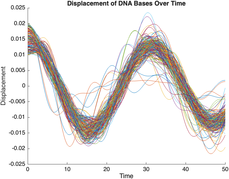
The results are visualized using a plot that shows the displacements of each base over time . Key observations from the simulation include :
- Wave Propagation: The initial perturbations lead to wave-like dynamics along the segment, with visible propagation and reflection at the boundaries.
- Damping Effects: The inclusion of damping leads to a gradual reduction in the amplitude of the oscillations, indicating energy dissipation over time.
- Nonlinear Behavior: The nonlinear term influences the response, potentially stabilizing the system against large displacements or leading to complex dynamic patterns.
% 3D plot for displacement
figure;
[X, T] = meshgrid(1:numBases, tspan);
surf(X', T', x);
xlabel('Base Pair');
ylabel('Time');
zlabel('Displacement');
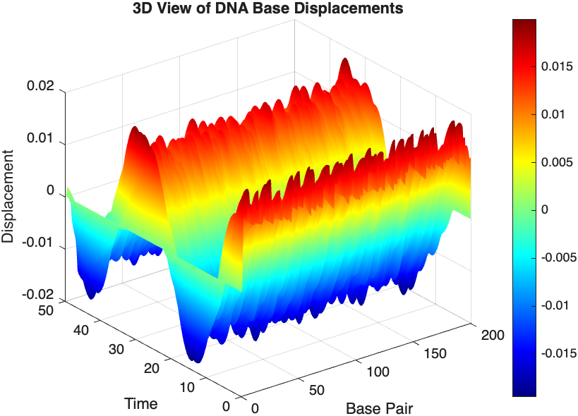
title('3D View of DNA Base Displacements');
colormap('jet');
shading interp;
colorbar; % Adds a color bar to indicate displacement magnitude
% Snapshot visualization at a specific time
snapshotTime = 40; % Desired time for the snapshot
[~, snapshotIndex] = min(abs(tspan - snapshotTime)); % Find closest index
snapshotSolution = x(:, snapshotIndex); % Extract displacement at the snapshot time
% Plotting the snapshot
figure;
stem(1:numBases, snapshotSolution, 'filled'); % Discrete plot using stem
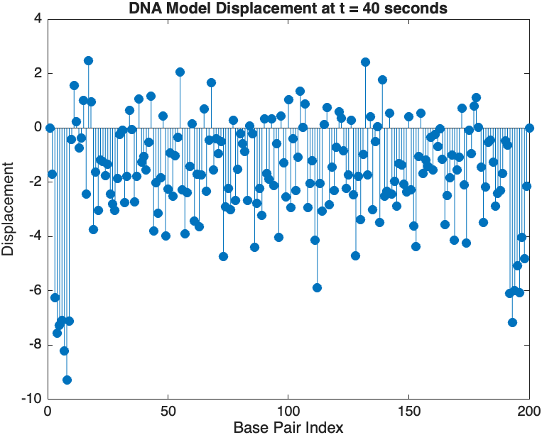
title(sprintf('DNA Model Displacement at t = %d seconds', snapshotTime));
xlabel('Base Pair Index');
ylabel('Displacement');
% Time vector for detailed sampling
tDetailed = 0:0.5:50; % Detailed time steps
% Initialize an empty array to hold the data
data = [];
% Generate the data for 3D plotting
for i = 1:numBases
% Interpolate to get detailed solution data for each base pair
detailedSolution = interp1(tspan, x(i, :), tDetailed);
% Concatenate the current base pair's data to the main data array
data = [data; repmat(i, length(tDetailed), 1), tDetailed', detailedSolution'];
end
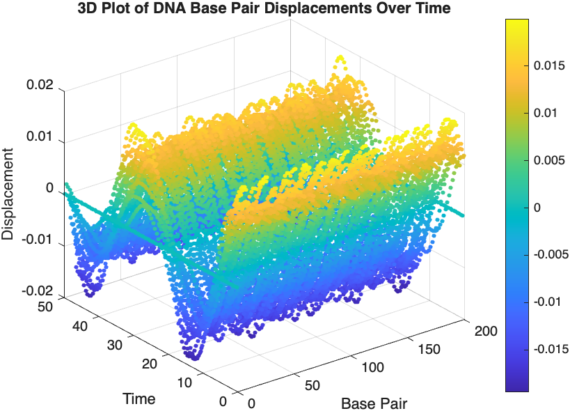
% 3D Plot
figure;
scatter3(data(:,1), data(:,2), data(:,3), 10, data(:,3), 'filled');
xlabel('Base Pair');
ylabel('Time');
zlabel('Displacement');
title('3D Plot of DNA Base Pair Displacements Over Time');
colorbar; % Adds a color bar to indicate displacement magnitude
また、以下のリストから Web サイトを選択することもできます。
南北アメリカ
- América Latina (Español)
- Canada (English)
- United States (English)
ヨーロッパ
- Belgium (English)
- Denmark (English)
- Deutschland (Deutsch)
- España (Español)
- Finland (English)
- France (Français)
- Ireland (English)
- Italia (Italiano)
- Luxembourg (English)
- Netherlands (English)
- Norway (English)
- Österreich (Deutsch)
- Portugal (English)
- Sweden (English)
- Switzerland
- United Kingdom(English)
アジア太平洋地域
- Australia (English)
- India (English)
- New Zealand (English)
- 中国
- 日本Japanese (日本語)
- 한국Korean (한국어)