結果:
The line integral  , where C is the boundary of the square
  oriented counterclockwise, can be evaluated in two ways:
, where C is the boundary of the square Using the definition of the line integral:
% Initialize the integral sum
integral_sum = 0;
% Segment C1: x = -1, y goes from -1 to 1
y = linspace(-1, 1);
x = -1 * ones(size(y));
dy = diff(y);
integral_sum = integral_sum + sum(-x(1:end-1) .* dy);
% Segment C2: y = 1, x goes from -1 to 1
x = linspace(-1, 1);
y = ones(size(x));
dx = diff(x);
integral_sum = integral_sum + sum(y(1:end-1).^2 .* dx);
% Segment C3: x = 1, y goes from 1 to -1
y = linspace(1, -1);
x = ones(size(y));
dy = diff(y);
integral_sum = integral_sum + sum(-x(1:end-1) .* dy);
% Segment C4: y = -1, x goes from 1 to -1
x = linspace(1, -1);
y = -1 * ones(size(x));
dx = diff(x);
integral_sum = integral_sum + sum(y(1:end-1).^2 .* dx);
disp(['Direct Method Integral: ', num2str(integral_sum)]);
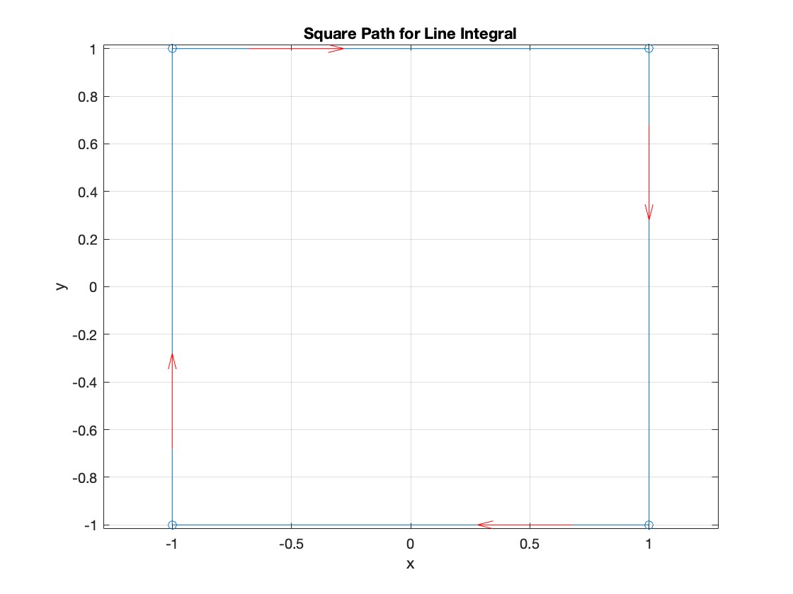
Plotting the square path
% Define the square's vertices
vertices = [-1 -1; -1 1; 1 1; 1 -1; -1 -1];
% Plot the square
figure;
plot(vertices(:,1), vertices(:,2), '-o');
title('Square Path for Line Integral');
xlabel('x');
ylabel('y');
grid on;
axis equal;
% Add arrows to indicate the path direction (counterclockwise)
hold on;
for i = 1:size(vertices,1)-1
% Calculate direction
dx = vertices(i+1,1) - vertices(i,1);
dy = vertices(i+1,2) - vertices(i,2);
% Reduce the length of the arrow for better visibility
scale = 0.2;
dx = scale * dx;
dy = scale * dy;
% Calculate the start point of the arrow
startx = vertices(i,1) + (1 - scale) * dx;
starty = vertices(i,2) + (1 - scale) * dy;
% Plot the arrow
quiver(startx, starty, dx, dy, 'MaxHeadSize', 0.5, 'Color', 'r', 'AutoScale', 'off');
end
hold off;
Apply Green's Theorem for the line integral
% Define the partial derivatives of P and Q
f = @(x, y) -1 - 2*y; % derivative of -x with respect to x is -1, and derivative of y^2 with respect to y is 2y
% Compute the double integral over the square [-1,1]x[-1,1]
integral_value = integral2(f, -1, 1, 1, -1);
disp(['Green''s Theorem Integral: ', num2str(integral_value)]);
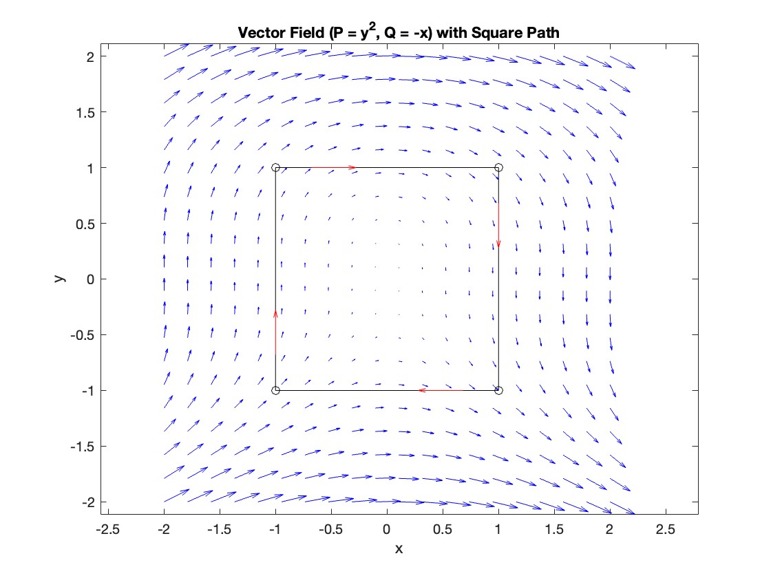
Plotting the vector field related to Green’s theorem
% Define the grid for the vector field
[x, y] = meshgrid(linspace(-2, 2, 20), linspace(-2 ,2, 20));
% Define the vector field components
P = y.^2; % y^2 component
Q = -x; % -x component
% Plot the vector field
figure;
quiver(x, y, P, Q, 'b');
hold on; % Hold on to plot the square on the same figure
% Define the square's vertices
vertices = [-1 -1; -1 1; 1 1; 1 -1; -1 -1];
% Plot the square path
plot(vertices(:,1), vertices(:,2), '-o', 'Color', 'k'); % 'k' for black color
title('Vector Field (P = y^2, Q = -x) with Square Path');
xlabel('x');
ylabel('y');
axis equal;
% Add arrows to indicate the path direction (counterclockwise)
for i = 1:size(vertices,1)-1
% Calculate direction
dx = vertices(i+1,1) - vertices(i,1);
dy = vertices(i+1,2) - vertices(i,2);
% Reduce the length of the arrow for better visibility
scale = 0.2;
dx = scale * dx;
dy = scale * dy;
% Calculate the start point of the arrow
startx = vertices(i,1) + (1 - scale) * dx;
starty = vertices(i,2) + (1 - scale) * dy;
% Plot the arrow
quiver(startx, starty, dx, dy, 'MaxHeadSize', 0.5, 'Color', 'r', 'AutoScale', 'off');
end
hold off;