生体信号のウェーブレット解析

MODWT を使用した心電図における R 波検出

QRS 群は、心電図 (ECG) 波形の 3 つの偏位で構成されます。QRS 群は、左右の心室の脱分極を反映するもので、人間の ECG の最も顕著な特徴です。

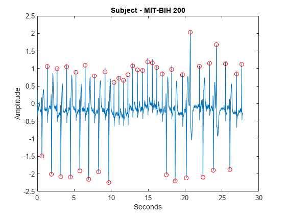
ECG 波形を読み込み、プロットします。この波形は、2 人以上の心臓専門医によって、QRS 群の R ピークに注釈が付けられています。ECG データと注釈は、MIT-BIH Arrhythmia Database から取得されたものです。データは 360 Hz でサンプリングされています。

load mit200
figure
plot(tm,ecgsig)
hold on
plot(tm(ann),ecgsig(ann),'ro')
xlabel('Seconds')
ylabel('Amplitude')
title('Subject - MIT-BIH 200')

ウェーブレットを使用して、R-R 間隔推定などのアプリケーションに使用する自動 QRS 検出器を構築できます。

ウェーブレットを一般的な特徴検出器として使用する場合、重要な点が 2 つあります。

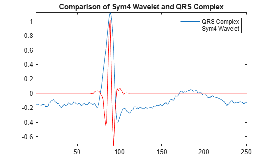
'sym4' ウェーブレットは QRS 群に似ているので、QRS 検出に適しています。これを明確に示すため、QRS 群を抽出し、その結果を膨張および平行移動した 'sym4' ウェーブレットとともにプロットして比較します。

qrsEx = ecgsig(4560:4810);
fb = dwtfilterbank('Wavelet','sym4','SignalLength',numel(qrsEx),'Level',3);
psi = wavelets(fb);
figure
plot(qrsEx)
hold on
plot(-2*circshift(psi(3,:),[0 -38]),'r')
axis tight
legend('QRS Complex','Sym4 Wavelet')
title('Comparison of Sym4 Wavelet and QRS Complex')
hold off

最大重複離散ウェーブレット変換 (MODWT) を使用して、ECG 波形内の R ピークを強調します。MODWT は非間引き離散ウェーブレット変換で、任意のサンプル サイズを処理します。

まず、既定の 'sym4' ウェーブレットを使用して、レベル 5 まで ECG 波形を分解します。次に、スケール 4 および 5 のウェーブレット係数のみを使用して、周波数局在型のバージョンの ECG 波形を再構築します。これらのスケールは、次の近似周波数帯域に対応します。

これは上記の通過帯域をカバーし、QRS エネルギーを最大化します。

wt = modwt(ecgsig,5);
wtrec = zeros(size(wt));
wtrec(4:5,:) = wt(4:5,:);
y = imodwt(wtrec,'sym4');

ウェーブレット係数から構築した信号 Approximation の絶対値の 2 乗を使用し、ピーク検出アルゴリズムを利用して R ピークを特定します。

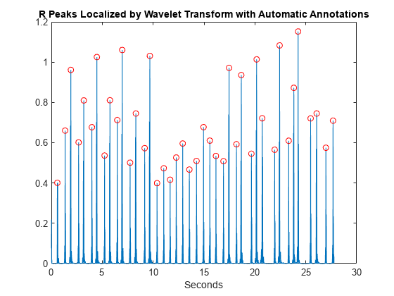
Signal Processing Toolbox™ がある場合、findpeaks を使用してピークの位置を特定できます。ウェーブレット変換を使用して取得した R ピーク波形をプロットし、自動検出したピークの位置で注釈を付けます。

y = abs(y).^2;
[qrspeaks,locs] = findpeaks(y,tm,'MinPeakHeight',0.35,...
    'MinPeakDistance',0.150);
figure
plot(tm,y)
hold on
plot(locs,qrspeaks,'ro')
xlabel('Seconds')
title('R Peaks Localized by Wavelet Transform with Automatic Annotations')

R ピーク波形に専門家の注釈を追加します。自動ピーク検出の時間は、本当のピークの 150 msec 以内 ($$\pm 75$$ msec) であれば正確と考えられます。

plot(tm(ann),y(ann),'k*')
title('R peaks Localized by Wavelet Transform with Expert Annotations')

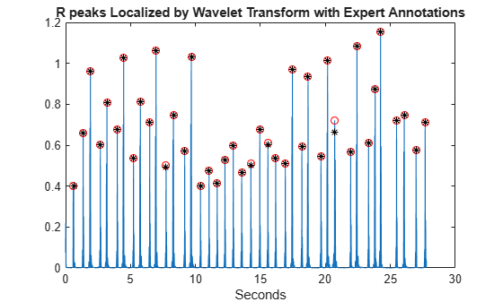
コマンド ラインで、tm(ann) および locs の値を比較できます。これらは、それぞれ専門家による時間と自動ピーク検出の時間です。ウェーブレット変換を使用して R ピークを強調した結果、ヒット率は 100%、誤検知はなしとなっています。ウェーブレット変換を使用して計算した心拍数は 88.60 bpm (1 分あたりの回数) です。これに対して、注釈付き波形では 88.72 bpm です。

元のデータの振幅の 2 乗で処理してみると、R ピークを分離するウェーブレット変換の機能によって検出の問題がかなり容易になることがわかります。生データで処理すると、10.4 秒のあたりで S 波のピークの 2 乗が R 波のピークを上回るときなど、誤認が生じる可能性があります。

figure
plot(tm,ecgsig,'k--')
hold on
plot(tm,y,'r','linewidth',1.5)
plot(tm,abs(ecgsig).^2,'b')
plot(tm(ann),ecgsig(ann),'ro','markerfacecolor',[1 0 0])
set(gca,'xlim',[10.2 12])
legend('Raw Data','Wavelet Reconstruction','Raw Data Squared', ...
    'Location','SouthEast')
xlabel('Seconds')

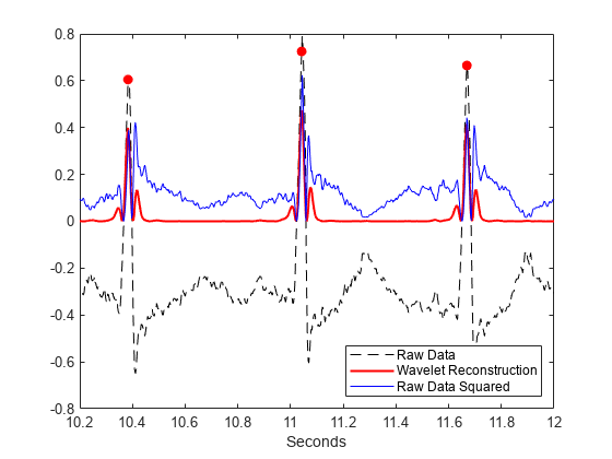
生データの振幅の 2 乗に findpeaks を使用すると、12 の誤検知が発生します。

[qrspeaks,locs] = findpeaks(ecgsig.^2,tm,'MinPeakHeight',0.35,...
    'MinPeakDistance',0.150);

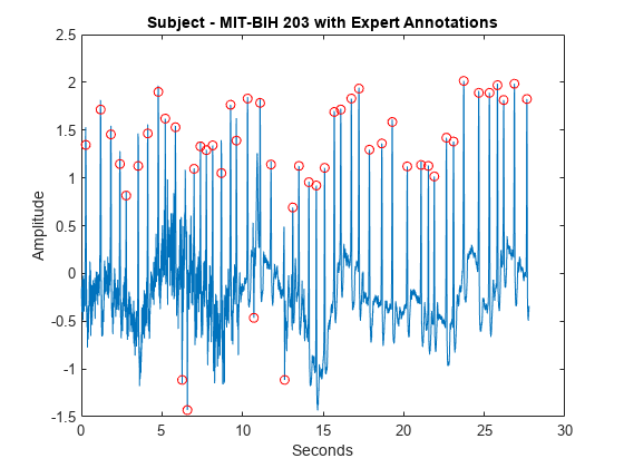
R ピークの極性の切り替わりに加え、ECG は頻繁にノイズによって破損します。

load mit203
figure
plot(tm,ecgsig)
hold on
plot(tm(ann),ecgsig(ann),'ro')
xlabel('Seconds')
ylabel('Amplitude')
title('Subject - MIT-BIH 203 with Expert Annotations')

MODWT を使用して R ピークを分離します。findpeaks を使用してピークの位置を特定します。R ピーク波形を、専門家の注釈および自動注釈とともにプロットします。

wt = modwt(ecgsig,5);
wtrec = zeros(size(wt));
wtrec(4:5,:) = wt(4:5,:);
y = imodwt(wtrec,'sym4');
y = abs(y).^2;
[qrspeaks,locs] = findpeaks(y,tm,'MinPeakHeight',0.1,...
    'MinPeakDistance',0.150);
figure
plot(tm,y)
title('R-Waves Localized by Wavelet Transform')
hold on
hwav = plot(locs,qrspeaks,'ro');
hexp = plot(tm(ann),y(ann),'k*');
xlabel('Seconds')
legend([hwav hexp],'Automatic','Expert','Location','NorthEast')

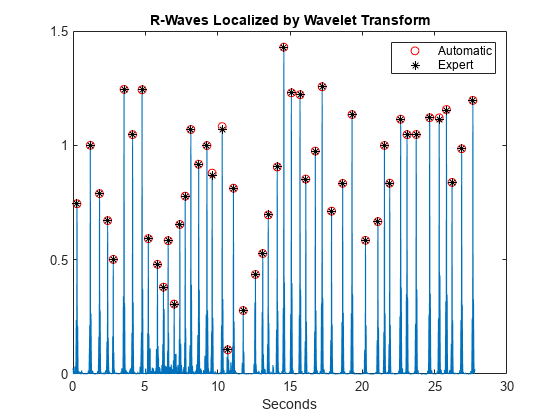
ヒット率は再び 100% となり、偽警報 は 0 です。

前の例では、modwtから構築した信号 Approximation に基づいて、非常にシンプルなウェーブレット QRS 検出器を使用しました。その目的は信号成分を分離するウェーブレット変換の機能を示すことであり、最もロバストなウェーブレット変換ベースの QRS 検出器の構築を目指したものではありません。たとえば、ウェーブレット変換が信号のマルチスケール解析を提供するという事実を利用して、ピーク検出を強化できます。専門家によって注釈が付けられた R ピークの時間とともにプロットされたスケール 4 および 5 の振幅二乗ウェーブレットの Detail を調べます。レベル 4 の Detail は、可視化のためにシフトされています。

ecgmra = modwtmra(wt);
figure
plot(tm,ecgmra(5,:).^2,'b')
hold on
plot(tm,ecgmra(4,:).^2+0.6,'b')
set(gca,'xlim',[14.3 25.5])
timemarks = repelem(tm(ann),2);
N = numel(timemarks);
markerlines = reshape(repmat([0;1],1,N/2),N,1);
h = stem(timemarks,markerlines,'k--');
h.Marker = 'none';
set(gca,'ytick',[0.1 0.6]);
set(gca,'yticklabels',{'D5','D4'})
xlabel('Seconds')
title('Magnitude-Squared Level 4 and 5 Details')

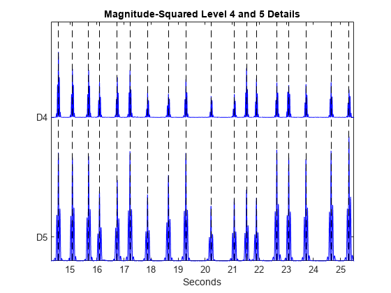
レベル 4 とレベル 5 の Detail のピークが同時に発生する傾向があることがわかります。複数のスケールからの情報を同時に使用することで、より高度なウェーブレット ピーク検出アルゴリズムを利用できます。

脳ダイナミクスの時変ウェーブレット コヒーレンス解析

フーリエ領域コヒーレンスは、周波数の関数として、2 つの定常過程間の線形相関を 0 から 1 のスケールで測定するための確立された手法です。ウェーブレットでは、データについての、時間とスケール (周波数) での局所情報が提供されるため、ウェーブレットベースのコヒーレンスを使用すると、周波数の関数として時変相関を測定できます。つまり、非定常過程に適したコヒーレンス測定というわけです。

これを説明するために、2 人の被験者から取得した近赤外線分光法 (NIRS) データを調べます。NIRS は、酸素化ヘモグロビンおよび脱酸素化ヘモグロビンの異なる吸収の特性を利用して、脳の活動を測定します。データは Cui, Bryant & Reiss (2012) によるもので、この例のために著者に提供していただきました。記録部位は両被験者の上前頭皮質でした。データは 10 Hz でサンプリングされます。

実験では、被験者はタスクに対して協力と競争を繰り返しました。タスクの周期は 7 秒でした。

load NIRSData
figure
plot(tm,[NIRSData(:,1) NIRSData(:,2)])
legend('Subject 1','Subject 2','Location','NorthWest')
xlabel('Seconds')
title('NIRS Data')
grid on

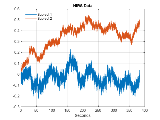
時間領域データを調べても、個々の時系列にどの振動が存在し、両方のデータ セットにどの振動が共通しているかは明らかではありません。ウェーブレット解析を使用して、両方の質問に答えます。

cwt(NIRSData(:,1),10,'bump')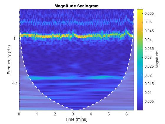

figure
cwt(NIRSData(:,2),10,'bump')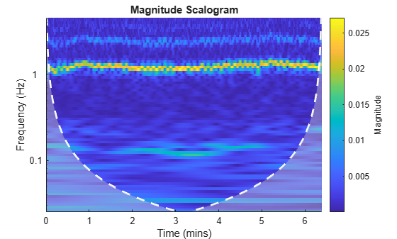

CWT 解析では、両方のデータセットの 1 Hz 付近で強い周波数変調振動が示されています。これらは、2 人の被験者の心周期によるものです。さらに、両方のデータセットの 0.15 Hz 付近で弱い振動があるように見えます。このアクティビティは、被験者 2 よりも被験者 1 において、より強く均一です。ウェーブレット コヒーレンスを使用することで、2 つの時系列に共存する弱い振動の検出を強化できます。

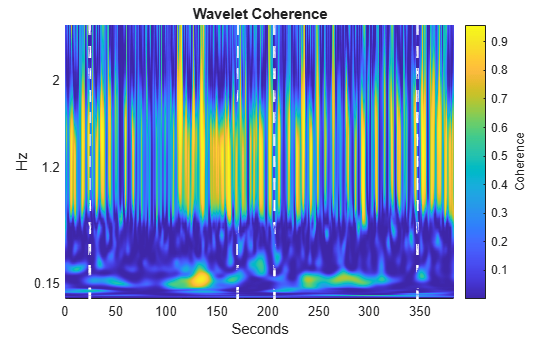
[wcoh,~,F] = wcoherence(NIRSData(:,1),NIRSData(:,2),10);
figure
surf(tm,F,abs(wcoh).^2); view(0,90)
shading interp
axis tight
hc = colorbar;
hc.Label.String = 'Coherence';
title('Wavelet Coherence')
xlabel('Seconds')
ylabel('Hz')
ylim([0 2.5])
set(gca,'ytick',[0.15 1.2 2])

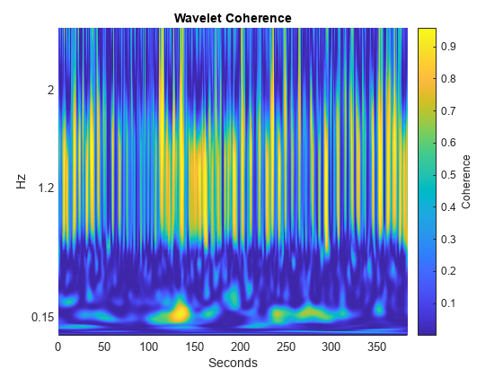
ウェーブレット コヒーレンスの 0.15 Hz 付近に強い相関関係があります。これは実験タスクに対応する周波数帯域にあり、被験者 2 人の脳の活動における、タスクに関連したコヒーレントな振動を表しています。2 つのタスク周期を示す時間マーカーをプロットに追加します。タスク間の期間は休止期間です。

taskbd = [245 1702 2065 3474];
tvec = repelem(tm(taskbd),2);
yvec = [0 max(F)]';
yvec = reshape(repmat(yvec,1,4),8,1);
hold on
stemPlot = stem(tvec,yvec,'w--','linewidth',2);
stemPlot.Marker = 'none';

この例では、cwtを使用し、個々の NIRS 時系列の時間-周波数解析を取得してプロットしました。この例ではまた、wcoherenceを使用し、2 つの時系列のウェーブレット コヒーレンスを取得しました。多くの場合、ウェーブレット コヒーレンスを使用すると、2 つの時系列において、個々の系列では非常に弱い場合があるコヒーレントな振動動作を検出できます。このデータのウェーブレット コヒーレンス解析の詳細については、Cui, Bryant, & Reiss (2012) を参照してください。

CWT を使用した耳音響放射データの時間-周波数解析

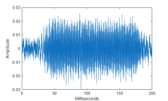
耳音響放射 (OAE) は蝸牛 (内耳) から発せられる狭帯域振動信号で、これがあることは正常な聴力を示します。サンプル OAE データをいくつか読み込んでプロットします。データは 20 kHz でサンプリングされます。

load dpoae
figure
plot(t.*1000,dpoaets)
xlabel('Milliseconds')
ylabel('Amplitude')

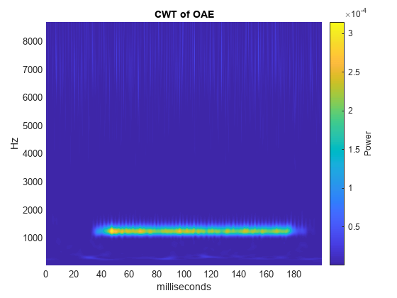
この放射は 25 ミリ秒から開始して 175 ミリ秒で終了するスティミュラスによって誘発されました。実験パラメーターに基づき、放射の周波数は 1230 Hz になります。時間と周波数の関数として CWT を取得してプロットします。オクターブあたりの音の数が 16 である既定の解析 Morse ウェーブレットを使用します。補助関数 helperCWTTimeFreqPlot を使用して、CWT をプロットします。補助関数は、この例と同じフォルダーにあります。

[dpoaeCWT,f] = cwt(dpoaets,2e4,'VoicesPerOctave',16);
helperCWTTimeFreqPlot(dpoaeCWT,t.*1000,f,...
    'surf','CWT of OAE','milliseconds','Hz')

OAE の時間発展は、周波数が 1230 Hz に最も近い CWT 係数を求め、その振幅を時間の関数として調べることで検証できます。誘発スティミュラスの開始と終了を指定する時間マーカーと共に振幅をプロットします。

[~,idx1230] = min(abs(f-1230));
cfsOAE = dpoaeCWT(idx1230,:);
plot(t.*1000,abs(cfsOAE))
hold on
AX = gca;
plot([25 25],[AX.YLim(1) AX.YLim(2)],'r')
plot([175 175],[AX.YLim(1) AX.YLim(2)],'r')
xlabel('msec')
title('CWT Coefficient Magnitudes')

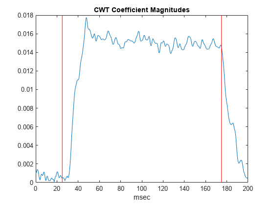
誘発スティミュラスのオンセットと OAE との間にいくらかの遅延があります。誘発スティミュラスが終了すると、OAE はすぐに振幅が減衰し始めます。

放射を分離するもう 1 つの方法は、逆 CWT を使用して時間領域で周波数局在型の Approximation を再構成することです。

1150 ～ 1350 Hz の周波数に対応する CWT 係数を抽出して、周波数局在型の放射の Approximation を構成します。これらの係数を使用して、CWT を反転します。誘発スティミュラスの開始と終了を示す再構成とマーカーと共に元のデータをプロットします。

frange = [1150 1350];
xrec = icwt(dpoaeCWT,[],f,frange);
figure
plot(t.*1000,dpoaets)
hold on
plot(t.*1000,xrec,'r')
AX = gca;
ylimits = AX.YLim;
plot([25 25],ylimits,'k')
plot([175 175],ylimits,'k')
grid on
xlabel('Milliseconds')
ylabel('Amplitude')
title('Frequency-Localized Reconstruction of Emission')

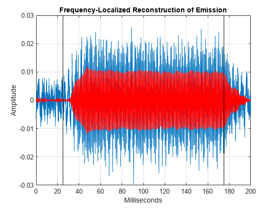
時間領域データでは、誘発スティミュラスの適用時と終了時に放射が増減するようすをはっきりと確認できます。

ここで重要な点は、再構成には周波数の範囲が選択された場合でも、解析ウェーブレット変換は実際には放射の正確な周波数を符号化することです。これを示すために、解析 CWT から再構成された放射の Approximation のフーリエ変換を使用します。

xdft = fft(xrec);
freq = 0:2e4/numel(xrec):1e4;
xdft = xdft(1:numel(xrec)/2+1);
figure
plot(freq,abs(xdft))
xlabel('Hz')
ylabel('Magnitude')
title('Fourier Transform of CWT-Based Signal Approximation')

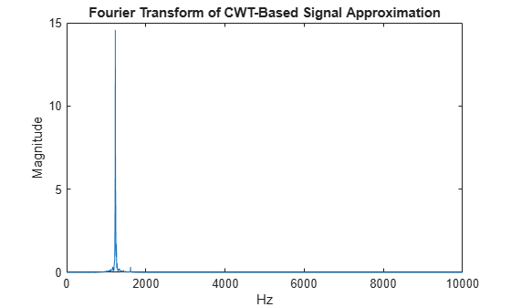
[~,maxidx] = max(abs(xdft));
fprintf('The frequency is %4.2f Hz\n',freq(maxidx))

The frequency is 1230.00 Hz

この例では、cwt を使用して OAE データの時間-周波数解析を取得し、icwtを使用して信号の周波数局在型の Approximation を取得しました。

参考文献

Cui, X., Bryant, D.M., and Reiss. A.L. "NIRS-Based hyperscanning reveals increased interpersonal coherence in superior frontal cortex during cooperation", Neuroimage, 59(3), 2430-2437, 2012.

Goldberger AL, Amaral LAN, Glass L, Hausdorff JM, Ivanov PCh, Mark RG, Mietus JE, Moody GB, Peng C-K, Stanley HE. "PhysioBank, PhysioToolkit, and PhysioNet: Components of a New Research Resource for Complex Physiologic Signals." Circulation 101(23):e215-e220, 2000. http://circ.ahajournals.org/cgi/content/full/101/23/e215

Mallat, S."A Wavelet Tour of Signal Processing:The Sparse Way", Academic Press, 2009.

Moody, G.B. "Evaluating ECG Analyzers". http://www.physionet.org/physiotools/wfdb/doc/wag-src/eval0.tex

Moody GB, Mark RG. "The impact of the MIT-BIH Arrhythmia Database." IEEE Eng in Med and Biol 20(3):45-50 (May-June 2001).