孤立森による異常検出

孤立森の紹介

孤立森アルゴリズム[1]は、孤立木のアンサンブルを使用して異常を正常な点から分離することにより、異常を検出します。各孤立木を学習観測値の部分集合用に学習させ、非復元抽出します。このアルゴリズムでは、部分集合ごとにすべての観測値が個別の葉ノードに到達するまで、無作為に分岐変数および分岐位置を選択することにより、孤立木を成長させます。異常は数が少なく異なります。そのため、異常はルート ノードに近い個別の葉ノードに到達し、パスの長さ (ルート ノードから葉ノードまでの距離) が正常な点より短くなります。すべての孤立木に対するパスの平均長さを基に定義された異常スコアを使用して、異常を識別します。

外れ値の検出と新規性の検出には、関数 iforest、IsolationForest オブジェクト、およびオブジェクト関数 isanomaly を使用します。

• 外れ値検出 (学習データ中の異常を検出) — 関数 iforest を使用して、学習データ中の異常を検出します。関数 iforest は、IsolationForest オブジェクトをビルドし、学習データの異常インジケーターおよびスコアを返します。例については、外れ値の検出を参照してください。

• 新規性の検出 (汚染されていない学習データで新規のデータの異常を検出) — 汚染されていない学習データ (外れ値がないデータ) を iforest に渡して IsolationForest オブジェクトを作成し、このオブジェクトおよび新規データをオブジェクト関数 isanomaly に渡して新規のデータの異常を検出します。新規のデータの各観測値について、学習済み孤立森のルート ノードから葉ノードに到達するパスの平均長さが計算され、異常インジケーターおよび異常スコアが返されます。例については、新規性の検出を参照してください。

孤立森のパラメーター

孤立森アルゴリズムのパラメーターは、iforest の名前と値の引数を使用して指定できます。

• NumObservationsPerLearner (各孤立木の観測値の数) — 各孤立木が学習観測値の部分集合に対応します。それぞれの木について、iforest は min(N,256) 個の観測値を学習データから非復元抽出します。N は学習観測値の数です。密な異常、および正常な点に近い異常の検出に役立つため、孤立森アルゴリズムは小さい標本サイズで適切に機能します。ただし、N が小さい場合は標本サイズを変えて試してみる必要があります。例については、小さいデータの NumObservationsPerLearner の調査を参照してください。

• NumLearners (孤立木の数) — 既定では、関数 iforest は孤立森の孤立木を 100 個まで成長させます。これは、通常は 100 個の孤立木を成長させるまでにパスの平均長さが十分に収束するためです[1]。

異常スコア

孤立森アルゴリズムでは、パスの長さ h(x) を正規化することにより、観測値 x の異常スコア s(x) を計算します。

$$s(x)=2^{-\frac{E[h(x)]}{c(n)}},$$

ここで、E[h(x)] は孤立森中にある孤立木すべてに関するパスの平均長さで、c(n) は n 個の観測値の二分探索木で失敗した探索のパスの平均長さです。

• スコアは E[h(x)] が 0 に近づくにつれて 1 に近づきます。したがって、1 に近いスコア値は異常を示しています。

• スコアは E[h(x)] が n – 1 に近づくにつれて 0 に近づきます。また、スコアは E[h(x)] が c(n) に近づくとき 0.5 に近づきます。したがって、0.5 より小さく 0 に近いスコア値は正常な点を示しています。

異常インジケーター

iforest および isanomaly は、異常スコアがスコアのしきい値を超える観測値を異常として識別します。関数は入力データと同じ長さの logical ベクトルを返します。値 logical 1 (true) は、入力データの対応する行が異常であることを示します。

• iforest は、指定された比率 (名前と値の引数 ContaminationFraction) の学習観測値が異常として検出されるようにしきい値 (ScoreThreshold プロパティの値) を決定します。既定では、関数はすべての学習観測値を正常な観測値として扱います。

• isanomaly では、名前と値の引数 ScoreThreshold を使用してしきい値を指定できます。既定のしきい値は、孤立森に学習させたときに決定された値になります。

外れ値の検出と異常スコアの等高線のプロット

この例では、外れ値を含む生成された標本データを使用します。関数iforestを使用して、孤立森モデルに学習させて外れ値を検出します。その後、関数isanomalyを使用して標本データの周りの点の異常スコアを計算し、異常スコアの等高線図を作成します。

標本データの生成

ガウス型コピュラを使用して、二変量分布からランダムなデータ点を生成します。

rng("default")
rho = [1,0.05;0.05,1];
n = 1000;
u = copularnd("Gaussian",rho,n);

無作為に選択された 5% の観測値にノイズを追加して、それらの観測値を外れ値にします。

noise = randperm(n,0.05*n);
true_tf = false(n,1);
true_tf(noise) = true;
u(true_tf,1) = u(true_tf,1)*5;

孤立森の学習と外れ値の検出

関数iforestを使用して孤立森モデルに学習させます。学習観測値に含まれている異常の比率を 0.05 と指定します。

[f,tf,scores] = iforest(u,ContaminationFraction=0.05);

f はIsolationForestオブジェクトです。iforest は、学習データの異常インジケーター (tf) および異常スコア (scores) も返します。

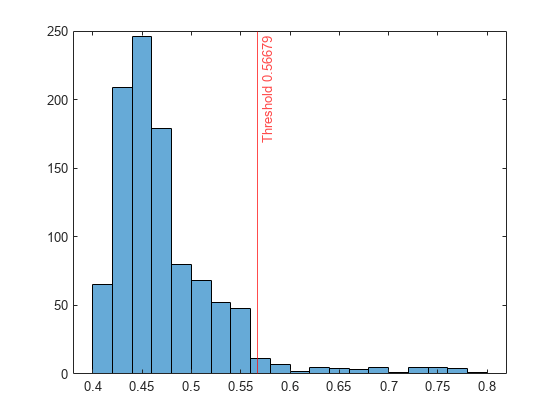
スコア値のヒストグラムをプロットします。指定した比率に対応するスコアのしきい値に垂直線を作成します。

histogram(scores)
xline(f.ScoreThreshold,"r-",join(["Threshold" f.ScoreThreshold]))

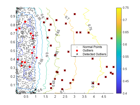
異常スコアの等高線のプロット

学習済み孤立森モデルと関数isanomalyを使用して、学習観測値の周りの 2 次元グリッド座標の異常スコアを計算します。

l1 = linspace(min(u(:,1),[],1),max(u(:,1),[],1));
l2 = linspace(min(u(:,2),[],1),max(u(:,2),[],1));
[X1,X2] = meshgrid(l1,l2);
[~,scores_grid] = isanomaly(f,[X1(:),X2(:)]);
scores_grid = reshape(scores_grid,size(X1,1),size(X2,2));

学習観測値の散布図と異常スコアの等高線図を作成します。真の外れ値と iforest で検出された外れ値にフラグを付けます。

idx = setdiff(1:1000,noise);
scatter(u(idx,1),u(idx,2),[],[0.5 0.5 0.5],".")
hold on
scatter(u(noise,1),u(noise,2),"ro","filled")
scatter(u(tf,1),u(tf,2),60,"kx",LineWidth=1)
contour(X1,X2,scores_grid,"ShowText","on")
legend(["Normal Points" "Outliers" "Detected Outliers"],Location="best")
colorbar
hold off

性能のチェック

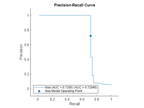
適合率-再現率曲線をプロットし、曲線の下の領域 (AUC) の値を計算して、iforest の性能をチェックします。rocmetricsオブジェクトを作成します。rocmetrics では、既定では偽陽性率と真陽性率 (つまり再現率) が計算されます。名前と値の引数 AdditionalMetrics を指定して、適合率の値 (つまり陽性の予測値) を追加で計算します。

rocObj = rocmetrics(true_tf,scores,true,AdditionalMetrics="PositivePredictiveValue");

rocmetrics の関数 plot を使用して曲線をプロットします。"y" 軸のメトリクスを適合率 (つまり陽性の予測値)、"x" 軸のメトリクスを再現率 (つまり真陽性率) として指定します。f.ScoreThreshold に対応するモデル操作点に塗りつぶされた円を表示します。関数 trapz の台形法を使用して適合率-再現率曲線の下の領域を計算し、その値を凡例に表示します。

r = plot(rocObj,YAxisMetric="PositivePredictiveValue",XAxisMetric="TruePositiveRate");
hold on
idx = find(rocObj.Metrics.Threshold>=f.ScoreThreshold,1,'last');
scatter(rocObj.Metrics.TruePositiveRate(idx), ...
    rocObj.Metrics.PositivePredictiveValue(idx), ...
    [],r.Color,"filled")
xyData = rmmissing([r.XData r.YData]);
auc = trapz(xyData(:,1),xyData(:,2));
legend(join([r.DisplayName " (AUC = " string(auc) ")"],""),"true Model Operating Point")
xlabel("Recall")
ylabel("Precision")
title("Precision-Recall Curve")
hold off

小さいデータの NumObservationsPerLearner の調査

それぞれの孤立木について、iforest は min(N,256) 個の観測値を学習データから非復元抽出します。N は学習観測値の数です。標本サイズが小さければ、密な異常、および正常な点に近い異常の検出に役立ちます。ただし、N が小さい場合は標本サイズを変えて試してみる必要があります。

この例では、さまざまな標本サイズの小さいデータで孤立森モデルに学習させ、異常スコアの値と標本サイズの関係をプロットし、識別された異常を可視化する方法を示します。

標本データの読み込み

フィッシャーのアヤメのデータ セットを読み込みます。

load fisheriris

データには、3 つの種のアヤメの花による 4 種類の測定値 (萼弁の長さ、萼弁の幅、花弁の長さ、花弁の幅) が含まれています。行列 meas には、150 本の花についての 4 つの測定値すべてが格納されています。

さまざまな標本サイズでの孤立森の学習

さまざまな標本サイズで孤立森モデルに学習させ、学習観測値の異常スコアを取得します。

s = NaN(150,150);
rng("default")
for i = 3: 150
    [~,~,s(:,i)] = iforest(meas,NumObservationsPerLearner=i);
end

観測値を平均スコアに基づいて 3 つのグループに分割し、異常スコアと標本サイズの関係を示すプロットを作成します。

score_threshold1 = 0.5;
score_threshold2 = 0.55;

m = mean(s,2,"omitnan");
ind1 = find(m < score_threshold1);
ind2 = find(m <= score_threshold2 & m >= score_threshold1);
ind3 = find(m > score_threshold2);

figure
t = tiledlayout(3,1);
nexttile
plot(s(ind1,:)')
title(join(["Observations with average score <  " score_threshold1]))
nexttile
plot(s(ind2,:)')
title(join(["Observations with average score in [" ...
    score_threshold1 " " score_threshold2 "]"]))
nexttile
plot(s(ind3,:)')
title(join(["Observations with average score >  " score_threshold2]))
xlabel(t,"Number of Observations for Each Tree")
ylabel(t,"Anomaly Score")

平均スコアの値が 0.5 未満の観測値では、標本サイズが大きくなるにつれて異常スコアが小さくなっています。平均スコアの値が 0.55 を超える観測値では、標本サイズが大きくなるにつれて異常スコアが大きくなり、標本サイズが 50 に達した時点でスコアがほぼ収束しています。

標本サイズが 50 と 100 の孤立森モデルを使用して、学習観測値の異常を検出します。学習観測値に含まれている異常の比率を 0.05 と指定します。

[f1,tf1,scores1] = iforest(meas,NumObservationsPerLearner=50, ...
    ContaminationFraction=0.05);
[f2,tf2,scores2] = iforest(meas,NumObservationsPerLearner=100, ...
    ContaminationFraction=0.05);

異常の観測値のインデックスを表示します。

find(tf1)

ans = 7×1

    14
    42
   110
   118
   119
   123
   132

find(tf2)

ans = 7×1

    14
    15
    16
   110
   118
   119
   132

2 つの孤立森モデルに共通の異常が 5 つあります。

異常の可視化

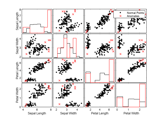
標本サイズが 50 の孤立森モデルについて、正常な点の観測値と異常の観測値を視覚的に比較します。関数gplotmatrixを使用して、変数の組み合わせごとにグループ化されたヒストグラムとグループ化された散布図の行列を作成します。

tf1 = categorical(tf1,[0 1],["Normal Points" "Anomalies"]);
predictorNames = ["Sepal Length" "Sepal Width" ...
    "Petal Length" "Petal Width"];
gplotmatrix(meas,[],tf1,"kr",".x",[],[],[],predictorNames)

高次元データの場合、重要な特徴量のみを使用してデータを可視化できます。t-SNE (t 分布型確率的近傍埋め込み) を使用して次元を減らしてからデータを可視化することもできます。

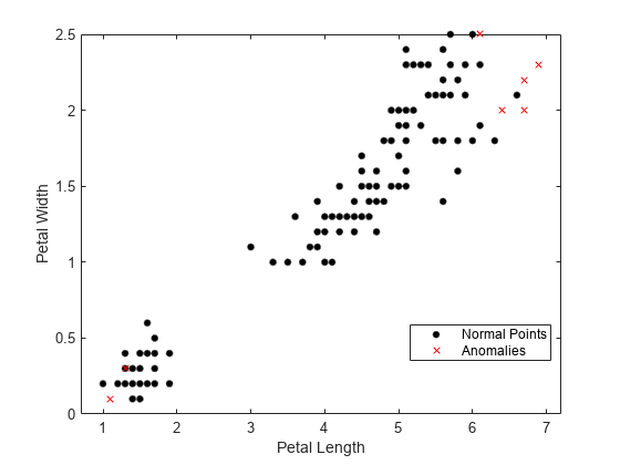
関数fsulaplacianで選択された最も重要な 2 つの特徴量を使用して観測値を可視化します。

idx = fsulaplacian(meas)

idx = 1×4

     3     4     1     2

gscatter(meas(:,idx(1)),meas(:,idx(2)),tf1,"kr",".x",[],"on", ...
    predictorNames(idx(1)),predictorNames(idx(2)))

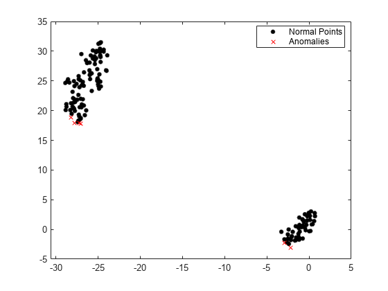
関数tsneを使用して次元を減らしてから観測値を可視化します。

Y = tsne(meas);
gscatter(Y(:,1),Y(:,2),tf1,"kr",".x")

参照

[1] Liu, F. T., K. M. Ting, and Z. Zhou. "Isolation Forest," 2008 Eighth IEEE International Conference on Data Mining. Pisa, Italy, 2008, pp. 413-422.

参考

iforest | IsolationForest | isanomaly

関連するトピック

• 教師なし異常検出