Safe PID Controller for Two Link Robot using High-Order Control Barrier Function

R2026b

Since R2026a

This example shows how to implement safety constraints using the High-Order Control Barrier Function block for a two-link robot with PID controller. The two-Link robot model and its corresponding dynamics are based on [1] and [2].

This example implements a high-order control barrier function in Simulink®. For an example that programmatically implements a control barrier function in MATLAB® , see Safe PID Tracking and Obstacle Avoidance Using Control Barrier Function.

Nonlinear Model and Objective

In this example, consider a two-link robot. The control objective is to move the robot tip from its starting point to a defined end point in the planar 2-D $x$-$y$ space. The tip position also has state constraints that you must consider when designing the controller. This figure shows the schematic of the two-link planar robot.

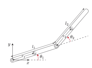
The robot configuration is defined by the joint angles ${\theta }_1$,${\theta }_2$ and the torques ${\tau }_1$ and ${\tau }_2$ applied at the joints to control the tip position. The state vector is:

$\zeta \left(t\right)=\left[\begin{array}{c}{\theta }_1\\ {\theta }_2\\ {\underset{}{\overset{\dot{}}{\theta }}}_1\left(t\right)\\ {\underset{}{\overset{\dot{}}{\theta }}}_2\left(t\right)\end{array}\right]$.

The following equations describe the robot dynamics.

$$\left[\begin{array}{cc}\alpha +2\beta \cos \left(\theta {}_2\right)& \delta +\beta \cos \left(\theta {}_2\right)\\ \delta +\beta \cos \left(\theta {}_2\right)& \delta \end{array}\right]\left[\begin{array}{c}\underset{}{\overset{¨}{{\theta }_1}}\\ \underset{}{\overset{¨}{{\theta }_2}}\end{array}\right]+\left[\begin{array}{cc}-\beta \sin \left({\theta }_2\right)\underset{}{\overset{\dot{}}{{\theta }_2}}& \beta \sin \left({\theta }_2\right)\left(\underset{}{\overset{\dot{}}{{\theta }_1}}+\underset{}{\overset{\dot{}}{{\theta }_2}}\right)\\ \beta \sin \left({\theta }_2\right)\underset{}{\overset{\dot{}}{{\theta }_1}}& 0\end{array}\right]\left[\begin{array}{c}\underset{}{\overset{\dot{}}{{\theta }_1}}\\ \underset{}{\overset{\dot{}}{{\theta }_2}}\end{array}\right]=\left[\begin{array}{c}{\tau }_1\\ {\tau }_2\end{array}\right]$$

Here:

$$\alpha =I_{\text{z1}}+I_{\text{z2}}+m_1{r}_1^2+m_2\left(l_1^2+r_2^2\right)$$

$$\beta =m_2{l}_1{r}_2$$

$$\delta =I_{\text{z2}}+m_2{r}_2^2$$

Define the physical parameters.

m1 = 3;         % Mass of link 1, kg
m2 = 2;         % Mass of link 2, kg
L1 = 0.3;       % Length of link 1, meters
L2 = 0.3;       % Length of link 2, meters

Calculate inertia terms for the Simulink® model.

r1 = L1/2;      % Length to centroid of link 1, meters
r2 = L2/2;      % Length to centroid of link 2, meters
Iz1 = m1*L1^2/12; % Moment of inertia of link 1, kg*m^2
Iz2 = m2*L2^2/12; % Moment of inertia of link 2, kg*m^2
beta = m2*L1*r2;
delta = Iz2 + m2*r2^2;
alpha = Iz1 + Iz2 + m1*r1^2 + m2*(L1^2 + r2^2);

The $x$-$y$ coordinates of the endpoints of link 1 and link 2, as functions of the link angles $\left[{\theta }_1,{\theta }_2\right]$, are defined as follows:

• Position of link 1 — $\begin{array}{l}{x}_1=L_1\cos \left({\theta }_1\right)\\ y_1=L_1\sin \left({\theta }_1\right)\end{array}$

• Position of link 2 — $\begin{array}{l}{x}_2=x_1+L_2\cos \left({\theta }_1+{\theta }_2\right)\\ y_2=y_1+L_2\sin \left({\theta }_1+{\theta }_2\right)\end{array}$

PID Controller for Two-Link Robot

For state-feedback control of the two-link robot, convert the start and end tip positions to joint angles using inverse kinematics for the two-link arm. Use the provided twoLinkInverseKinematics.m script to obtain joint angles from tip coordinates.

Specify the start position of tip of two-link robot as $\left[x_2\left(0\right),y_2\left(0\right)\right]$ to obtain the corresponding link angles $\left[{\theta }_1\left(0\right),{\theta }_2\left(0\right)\right]$.

InitialX = -0.5;
InitialY = -0.0496;
[InitialTheta1ref, InitialTheta2ref] = ...
    twoLinkInverseKinematics(InitialX,InitialY,L1,L2);

Similarly, specify the end position $\left[x_2\left(t_f\right),y_2\left(t_f\right)\right]$ to obtain corresponding link angles $\left[{\theta }_1\left(t_f\right),{\theta }_2\left(t_f\right)\right]$.

FinalX = 0.5;
FinalY = 0.2496;
[FinalTheta1ref, FinalTheta2ref] = ...
    twoLinkInverseKinematics(FinalX,FinalY,L1,L2);

Design the PID controllers to move the two-link robot from its initial orientation to the final orientation of the links. Implement the PID controllers as two decoupled channels. One for controlling angle ${\theta }_1$ of link 1, the other angle ${\theta }_2$ of link 2, as shown in the following figure.

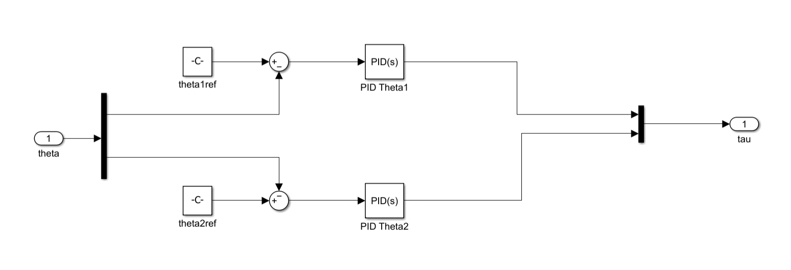
This example uses two PID controllers with gains tuned using the PID Tuner app. For more information on tuning PID controllers for Simulink® models, see Introduction to Model-Based PID Tuning in Simulink.

Results with Baseline PID

Open the model TwoLinkRobotWithPID, which includes the designed PID controllers for the two-link robot.

mdl = "TwoLinkRobotWithPID";
open_system(mdl)

Simulate the model.

out = sim(mdl);

% Extract the link angles and control signal
TwoLinkTheta1 = squeeze(out.theta1.Data);
TwoLinkTheta2 = squeeze(out.theta2.Data);
u_pid = out.u.data;

Plot the PID controller tracking performance.

figure
subplot(2,1,1)
hold on
plot(out.tout,TwoLinkTheta1,LineWidth=2)
plot(out.tout,FinalTheta1ref*ones(1,length(out.tout)), ...
    LineWidth=2,LineStyle="--")
legend("Theta1","Theta1_ref")
ylabel("theta1")
title("Two-Link Robot Angles vs Ref Angle")
subplot(2,1,2)
hold on
plot(out.tout,TwoLinkTheta2,LineWidth=2)
plot(out.tout,FinalTheta2ref*ones(1,length(out.tout)), ...
    LineWidth=2,LineStyle="--")
legend("Theta2","Theta2_ref")
xlabel("time (sec)")
ylabel("theta2")

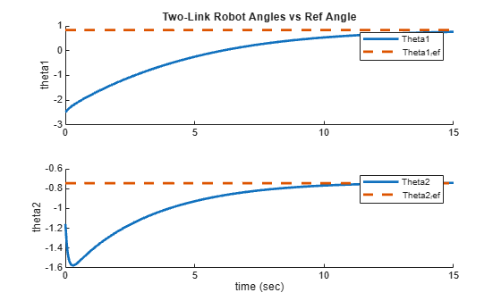
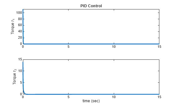
Plot the PID controller output.

figure
subplot(2,1,1)
plot(out.tout, u_pid(:,1),LineWidth=2)
ylabel("Torque \tau_1")
title("PID Control")
subplot(2,1,2)
plot(out.tout, u_pid(:,2),LineWidth=2)
xlabel("time (sec)")
ylabel("Torque \tau_2")

View the animation of the two-link robot under PID control as it moves from the specified start position to the end position.

PlotTwoLinkArm(TwoLinkTheta1,TwoLinkTheta2, ...
    InitialX,InitialY,FinalX,FinalY,L1,L2,-0.4)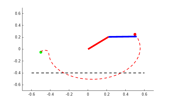

The standard PID controller does not provide a way to enforce safety constraints. The next section introduces control barrier functions, which add safety constraints to the baseline controller.

Safe Controller Using Control Barrier Function

A control barrier function (CBF) is a mathematical method that guarantees safety of a controlled system by ensuring the state remains within a defined safe region. It achieves this by imposing constraints on the control input at each time step, preventing the system from entering unsafe regions [3].

To introduce optimization-based safe controllers using CBF, consider a nonlinear, control-affine system defined as follows:

$\underset{}{\overset{\dot{}}{x}}=f\left(x\right)+g\left(x\right)u$.

For the given dynamical system and in the context of CBF, define a safe set $\mathcal{C}$as the set of all state values $x\left(t\right)$ that satisfy the condition $h\left(x\right)\ge 0$. Here, the smooth function $h\left(x\right)$ is the control barrier function.

You can construct a control barrier function $h\left(x\right)$ such that a state trajectory $x\left(t\right)\forall t>0$ that remains within the set $\mathcal{C}:h\left(x\right)>0$ is considered safe.

Given the control system and the safe set $\mathcal{C}$ defined by function $h\left(x\right)$, the safety condition is defined as follows:

For all control $u\left(t\right)$, ensure $\underset{}{\overset{\dot{}}{h}}\left(x,u\right)\ge -\gamma h\left(x\right)$.

Here, $\gamma$ is an extended class ${\mathcal{K}}_{\infty }$ function, and $\underset{}{\overset{\dot{}}{h}}\left(x,u\right)$ is the Lie derivative. For more details, see Enforce Safety Constraints with Control Barrier Functions.

Safe Control Synthesis Using CBF

Using the definition of the safe set, you can derive the safe control through an optimization routine.

Before that, review the concept of the Lie derivative of a CBF $h\left(x\right)$. The CBF is scalar function such that $h\left(x\right):{\mathbb{R}}^n\to \mathbb{R}$. The Lie derivative is the time derivative of $h\left(x\right)$ along the flow field given by the system dynamics $\underset{}{\overset{\dot{}}{x}}=f\left(x\right)+g\left(x\right)u$.

The Lie derivative is defined as:

$\underset{}{\overset{\dot{}}{h}}\left(x,u\right)=\frac{\partial h\left(x\right)}{\partial x}\underset{}{\overset{\dot{}}{x}}$.

Using the definition of the system dynamics, you can further simplify the Lie derivative as:

$\underset{}{\overset{\dot{}}{h}}\left(x,u\right)=\frac{\partial h\left(x\right)}{\partial x}f\left(x\right)+\frac{\partial h\left(x\right)}{\partial x}g\left(x\right)u$.

Hence, the safety condition is written as:

$L_{f}h\left(x\right)+L_{g}h\left(x\right)u\ge -\gamma h\left(x\right)$,

where $L_{f}h\left(x\right)=\frac{\partial h\left(x\right)}{\partial x}f\left(x\right)$ and $L_{g}h\left(x\right)=\frac{\partial h\left(x\right)}{\partial x}g\left(x\right)$

Using the defined inequality constraint, you can now compute the safe control $u^{*}$. To achieve this, consider the following quadratic programming (QP)-based controller that finds the minimum perturbation on $u$ as follows:

$$\begin{array}{l}{u}^{*}=\underset{u}{\min }\frac{1}{2}||u-u_0|{|}^2\\ s.t{L}_{f}h\left(x\right)+L_{g}h\left(x\right)u\ge -\gamma h\left(x\right),\end{array}$$

where $u_0$ is any designed baseline controller.

When the control term does not appear in the first-order Lie derivative of the CBF, you can use higher-order derivatives of the CBF. For the theory and derivation of high-order barrier functions, see [3] and Enforce Safety Constraints with Control Barrier Functions.

High-Order CBF for Two-Link Robot

For the two-link robot problem, you impose a safety constraint that prevents the tip of the second link from extending beyond the specified boundary $y_2=-0.4$ as shown in this figure.

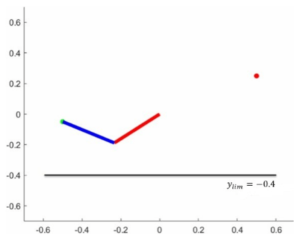
The control barrier function for the corresponding safety constraint is:

$h\left(y_2\right)=0.4+y_2\left(t\right)$.

This barrier function models the safe and unsafe regions as follows:

$$\mathcal{C}=\{\begin{array}{ll}\infty >y_2>-0.4& :h\left(y_2\right)>0\left(\text{Safe}\right)\\ y_2=-0.4& :h\left(y_2\right)=0\left(\text{Safe}\text{boundary}\right)\\ y_2<-0.4& :h\left(y_2\right)<0\left(\text{Unsafe}\right)\end{array}$$

Using the Cartesian coordinates of the endpoint of the two-link robot, the control barrier function is:

$$h\left(\zeta \right)=0.4+{L_1\sin \left({\theta }_1\right)+L}_2\sin \left({\theta }_1+{\theta }_2\right)$$

Derive the Lie derivative of the CBF and form the QP problem for safe control synthesis.

The constraint equation for safe control is $\underset{}{\overset{\dot{}}{h}}\left(\zeta ,u\right)\ge -\gamma h\left(\zeta \right)$.

Take the first Lie derivative of the barrier function with respect to states of two-link robot.

$\begin{array}{l}\underset{}{\overset{\dot{}}{h}}\left(\zeta ,u\right)=\frac{\partial h}{\partial \zeta }\underset{}{\overset{\dot{}}{\zeta }}\\ \underset{}{\overset{\dot{}}{h}}\left(\zeta ,u\right)=L_{f}h=\left[\begin{array}{cccc}{L_1\cos \left({\theta }_1\right)+L}_2\cos \left({\theta }_1+{\theta }_2\right)& L_2\cos \left({\theta }_1+{\theta }_2\right)& 0& 0\end{array}\right]\left[\begin{array}{c}\underset{}{\overset{\dot{}}{{\theta }_1}}\\ \underset{}{\overset{\dot{}}{{\theta }_2}}\\ \underset{}{\overset{¨}{{\theta }_1}}\\ \underset{}{\overset{¨}{{\theta }_2}}\end{array}\right]\end{array}$

The first Lie derivative does not expose the control term $u\left(t\right)$. For safety constraints, the control input should appear linearly in the constraint equation. Therefore, take the second Lie derivative.

$$\begin{array}{l}\underset{}{\overset{¨}{h}}\left(\zeta ,u\right)=\frac{\partial L_{f}h}{\partial \zeta }\underset{}{\overset{\dot{}}{\zeta }}\\ \underset{}{\overset{¨}{h}}\left(\zeta ,u\right)=\left[\begin{array}{cccc}-\underset{}{\overset{\dot{}}{{\theta }_1}}{L}_1\sin \left({\theta }_1\right)-{\underset{}{\overset{\dot{}}{{\theta }_1}}L}_2\sin \left({\theta }_1+{\theta }_2\right)-{\underset{}{\overset{\dot{}}{{\theta }_2}}L}_2\sin \left({\theta }_1+{\theta }_2\right)& -{\underset{}{\overset{\dot{}}{{\theta }_1}}L}_2\sin \left({\theta }_1+{\theta }_2\right)-{\underset{}{\overset{\dot{}}{{\theta }_2}}L}_2\sin \left({\theta }_1+{\theta }_2\right)& {L_1\cos \left({\theta }_1\right)+L}_2\cos \left({\theta }_1+{\theta }_2\right)& L_2\cos \left({\theta }_1+{\theta }_2\right)\end{array}\right]\left[\begin{array}{c}\underset{}{\overset{\dot{}}{{\theta }_1}}\\ \underset{}{\overset{\dot{}}{{\theta }_2}}\\ \underset{}{\overset{¨}{{\theta }_1}}\\ \underset{}{\overset{¨}{{\theta }_2}}\end{array}\right]\end{array}$$

The second Lie derivative involves term $\left[\underset{}{\overset{¨}{{\theta }_1}},\underset{}{\overset{¨}{{\theta }_2}}\right]$. Therefore, the control term appears through system dynamics as follows:

$$\underset{}{\overset{¨}{h}}\left(\zeta ,u\right)=L_f^{2}h+L_g{L}_{f}hu$$

where $L_f^{2}h=\frac{\partial L_{f}h}{\partial \zeta }f\left(\zeta \right)$ and $L_g{L}_{f}h=\frac{\partial L_{f}h}{\partial \zeta }g\left(\zeta \right)$.

The plant model $f\left(\zeta \right)$ and $g\left(\zeta \right)$ are defined as follows

$f\left(\zeta \right)=\left[\begin{array}{cc}{I}_{2\times 2}& 0_{2\times 2}\\ 0_{2\times 2}& M\left(\zeta \right)\end{array}\right]$ and $g\left(\zeta \right)=\left[\begin{array}{c}{0}_{2\times 2}\\ G\left(\zeta \right)\end{array}\right]$

$M\left(\zeta \right)={\left[\begin{array}{cc}\alpha +2\beta \cos \left(\theta {}_2\right)& \delta +\beta \cos \left(\theta {}_2\right)\\ \delta +\beta \cos \left(\theta {}_2\right)& \delta \end{array}\right]}^{-1}\left[\begin{array}{cc}-\beta \sin \left({\theta }_2\right)\underset{}{\overset{\dot{}}{{\theta }_2}}& \beta \sin \left({\theta }_2\right)\left(\underset{}{\overset{\dot{}}{{\theta }_1}}+\underset{}{\overset{\dot{}}{{\theta }_2}}\right)\\ \beta \sin \left({\theta }_2\right)\underset{}{\overset{\dot{}}{{\theta }_1}}& 0\end{array}\right]$ , $G\left(\zeta \right)={\left[\begin{array}{cc}\alpha +2\beta \cos \left(\theta {}_2\right)& \delta +\beta \cos \left(\theta {}_2\right)\\ \delta +\beta \cos \left(\theta {}_2\right)& \delta \end{array}\right]}^{-1}$ and $u=\left[\begin{array}{c}{\tau }_1\\ {\tau }_2\end{array}\right]$

The second-order CBF safety constraints and QP formulation for the two-link robot are:

$$\begin{array}{l}{u}^{*}=\underset{u}{\min }\frac{1}{2}{\Vert u-u_{\text{pid}}\Vert }^2\\ s.t{L}_f^{2}h+L_g{L}_{f}hu+{\gamma }_{1}h+{\gamma }_2{L}_{f}h\ge 0\end{array}$$

You can implement this derived formulation using the High-Order Control Barrier Function block.

High-Order CBF Results

The TwoLinkRobotWithHOCBF model contains the PID controllers, the plant dynamics, and the high-order control barrier function implementation.

mdl = "TwoLinkRobotWithHOCBF";
open_system(mdl)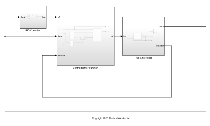

To view the CBF implementation, open the Control Barrier Function subsystem. The model implements the known CBF using a MATLAB Function block, and the High-Order Control Barrier Function block enforces the constraint function.

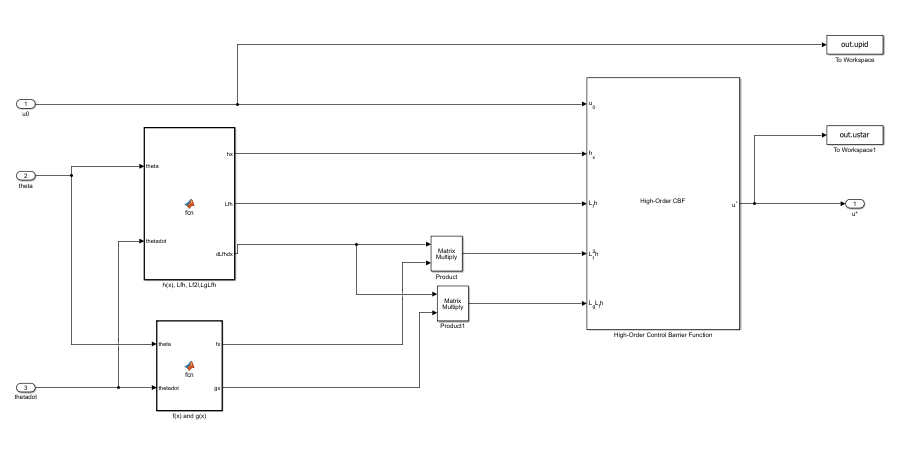
Simulate the model and plot the results.

out = sim(mdl);

Extract the link angles and control signal.

TwoLinkTheta1 = squeeze(out.theta1.Data);
TwoLinkTheta2 = squeeze(out.theta2.Data);
u_hocbf = squeeze(out.ustar.data);
u_pid = squeeze(out.upid.data);

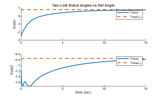
Plot the link angles.

figure
subplot(2,1,1)
hold on
plot(out.tout,TwoLinkTheta1,LineWidth=2)
plot(out.tout,FinalTheta1ref*ones(1,length(out.tout)), ...
    LineWidth=2,LineStyle="--")
legend("Theta1","Theta1_{ref}")
ylabel("theta1")
title("Two-Link Robot Angles vs Ref Angle")
subplot(2,1,2)
hold on
plot(out.tout,TwoLinkTheta2,LineWidth=2)
plot(out.tout,FinalTheta2ref*ones(1,length(out.tout)), ...
    LineWidth=2,LineStyle="--")
legend("Theta2","Theta2_{ref}")
xlabel("time (sec)")
ylabel("theta2")

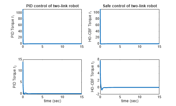
Compare the high-order CBF constrained control with the baseline PID control.

figure
subplot(2,2,1)
plot(out.tout,u_pid(1,:),LineWidth=2)
ylabel("PID Torque \tau_1")
title("PID control of two-link robot")
subplot(2,2,2)
plot(out.tout,u_hocbf(:,1),LineWidth=2)
ylabel("HO-CBF Torque \tau_1")
title("Safe control of two-link robot")
subplot(2,2,3)
plot(out.tout,u_pid(2,:),LineWidth=2)
ylabel("PID Torque \tau_2")
xlabel("time (sec)")
subplot(2,2,4)
plot(out.tout, u_hocbf(:,2),LineWidth=2)
ylabel("HO-CBF Torque \tau_2")
xlabel("time (sec)")

View the animation of the two-link robot under safe control, generated by the high-order CBF with the baseline PID control, as it moves from the specified start position to the end position.

PlotTwoLinkArm(TwoLinkTheta1,TwoLinkTheta2, ...
    InitialX,InitialY,FinalX,FinalY,L1,L2,-0.4)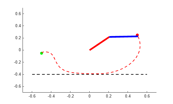

The High-Order Control Barrier Function block successfully constrains the tip of the two-link robot within the given safe state bounds.

Automatic Lie Derivative Generation Using Auto-Differentiation in MATLAB

Since R2026b

Hand-deriving Lie derivatives, especially for higher relative orders or more complex barrier functions, is time-consuming and error-prone.

If you can define functions for your barrier function and model dynamics, then you can programmatically generate Lie derivatives using a ControlBarrierFunction object and the generateLieDerivativeFcn function. This workflow uses automatic differentiation (auto‑diff) to trace the computational graph of a user‑supplied barrier function and model dynamics to produce Lie derivatives. For auto‑diff to work the barrier and model functions must be differentiable functions with respect to the state vector $x$.

Define Barrier Function

Create a ControlBarrierFunction object with four states, two inputs, one constraint, and a relative order of two. These values match the specifications in the High-Order Control Barrier Function block.

cbf = ControlBarrierFunction(4,2, ...
    NumOfConstraints=1, ...
    RelativeOrder=2);

A barrier function $h\left(x\right)$ is a smooth function whose nonnegative level set defines a safe region, and whose Lie‑derivative constraints are used to enforce that system trajectories remain inside the safe region.

• The first input to the barrier function must be the state x.

• You can optionally specify additional input parameters. In this example, specify the arm lengths L1 and L2.

• The output must be a scalar or NumOfConstraints-by-1 column vector.

Specify the barrier function as TwoLinkRobotBarrierFcn, which is a function on the MATLAB path.

cbf.Constraints.BarrierFcn = @(x) TwoLinkRobotBarrierFcn(x,L1,L2);

Define Model Function

The model function computes the control‑affine dynamics for the current state x and returns the drift f(x) and input matrix g(x).

• First input is the state x.

• Outputs are f and g, where f is an nx-by-1 column vector and g is an nx-by-nu matrix.

For this example, the model dynamics are defined in the TwoLinkModel function, which has the function signature [fx,gx] = TwoLinkModel(x).

Generate Lie Derivatives

Generate the Lie derivatives for the control barrier function using the model function.

cbf = generateLieDerivativeFcn(cbf,"TwoLinkModel");

Simulate Model

Open and simulate a Simulink model that uses the auto-generated Lie derivatives.

mdl = "TwoLinkRobot_withAutoDiff";
open_system(mdl);
out = sim(mdl);

Extract the link angles and control signal.

TwoLinkTheta1 = squeeze(out.theta1.Data);
TwoLinkTheta2 = squeeze(out.theta2.Data);
u_hocbf = squeeze(out.ustar.data);
u_pid = squeeze(out.upid.data);

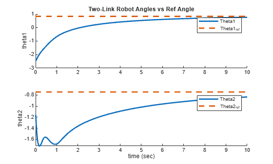
Plot the link angles

figure
subplot(2,1,1)
hold on
plot(out.tout,TwoLinkTheta1,LineWidth=2)
plot(out.tout,FinalTheta1ref*ones(1,length(out.tout)), ...
    LineWidth=2,LineStyle="--")
legend("Theta1","Theta1_{ref}")
ylabel("theta1")
title("Two-Link Robot Angles vs Ref Angle")
subplot(2,1,2)
hold on
plot(out.tout,TwoLinkTheta2,LineWidth=2)
plot(out.tout,FinalTheta2ref*ones(1,length(out.tout)), ...
    LineWidth=2,LineStyle="--")
legend("Theta2","Theta2_{ref}")
xlabel("time (sec)")
ylabel("theta2")

View the animation of the two-link robot for this simulation.

PlotTwoLinkArm(TwoLinkTheta1,TwoLinkTheta2, ...
    InitialX,InitialY,FinalX,FinalY,L1,L2,-0.4)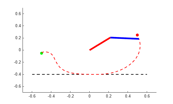

This system successfully constrains the tip of the two-link robot within the given safe state bounds.

Conclusion

This example demonstrates how to enforce safety for a two‑link planar robot using high‑order control barrier functions (HOCBF). A baseline PID controller with a second‑order CBF prevents the robot tip from crossing the specified unsafe boundary. The example also illustrates automated Lie‑derivative generation, which simplifies deriving higher‑order Lie derivatives for Simulink implementation. The HOCBF approach preserves nominal performance when possible and guarantees safety by enforcing input constraints at each time step.

References

[1] Murray, Richard M., Zexiang Li, and S. Shankar Sastry. A Mathematical Introduction to Robotic Manipulation. CRC Press, 1994.

[2] Seiler, Peter, Robert M. Moore, Chris Meissen, Murat Arcak, and Andrew Packard. “Finite Horizon Robustness Analysis of LTV Systems Using Integral Quadratic Constraints.” Automatica 100 (February 2019): 135–43. https://doi.org/10.1016/j.automatica.2018.11.009.

[3] Xiao, Wei, and Calin Belta. “High-Order Control Barrier Functions.” IEEE Transactions on Automatic Control 67, no. 7 (2022): 3655–62. https://doi.org/10.1109/TAC.2021.3105491.