Safe PID Tracking and Obstacle Avoidance Using Control Barrier Function

R2026b

This example shows how to implement safety constraints using the control barrier functions for control systems modeled in MATLAB®. The example implements a PID path tracking model for a Dubins car model.

Dubins Car Model and Dubins Path

The Dubins car is a simple vehicle model with state $q=\left[x,y,\theta \right]$, where ($x$,$y$) is the position and $\theta$ is the heading. The vehicle moves forward at constant speed $v$ [1] and is steered by a bounded steering command $u$ (here normalized to [-1, 1]). The kinematic equations are:

$$\begin{array}{l}\underset{}{\overset{\dot{}}{x}}=v*\cos \left(\theta \right)\\ \underset{}{\overset{\dot{}}{y}}=v*\sin \left(\theta \right)\\ \underset{}{\overset{\dot{}}{\theta }}=\frac{v}{r_{\min }}u\end{array}$$

The control steering input is bounded $-1\le u\le 1$ and produces the minimum turning radius $r_{\min }$, and $u=0$ yields straight-line motion.

Define the Dubins car parameters.

v = 2.0;           % Forward speed (m/s)
r_min = 3.0;       % Minimum turning radius (m)
dt = 0.05;         % Time step (s)

Dubins Path For Waypoints

A Dubins path is the shortest feasible trajectory for a vehicle that moves forward at constant speed and has a bounded curvature (minimum turning radius r_min) [1]. For waypoint navigation, you connect successive pose waypoints $\left[x,y,\theta \right]$ using a sequence of at most three primitive motions: straight (S), left turn at maximum curvature (L), and right turn at maximum curvature (R). The permitted combinations (LSL, LSR, RSL, RSR, RLR, LRL) are searched and the shortest valid sequence that respects minimum turn radius $r_{\min }$ is chosen.

When generating a reference mission from waypoints:

• Each consecutive pair of waypoints is converted to a Dubins path segment computed with the vehicle $r_{\min }$.

• Each segment yields a set of interpolated poses $\left[x,y,\theta \right]$ and a length; concatenating these points produces a smooth, kinematically-feasible reference path for the nonholonomic car.

• Using the heading at each waypoint allows continuous orientation along the path so controller (PID) can track both position and heading.

Set the waypoints for this example.

waypoints = [
    0,   0,   0;
    15,  10,  pi/4;
    30,   5,  0;
    40,  15,  pi/2;
    35,  25,  pi;
    ];

In this example the helper function generate_dubins_path uses the dubinsConnection function to compute the shortest Dubins path between consecutive waypoints and returns the interpolated reference trajectory. The dubinsConnection function requires Navigation Toolbox™ software.

[ref_path,total_path_length] = generate_dubins_path(waypoints,r_min);

PID Tracking Simulation

A baseline PID controller for the Dubins car provides a simple, robust lateral controller that commands a normalized steering value $u\in \left[-1,1\right]$ to minimize cross-track error (CTE) and heading error relative to a reference path. The PID controller treats longitudinal speed $v$ as constant and focuses on steering to drive the vehicle toward the nearest look-ahead reference pose.

The Cross-track error is defined as lateral distance from the vehicle position to the reference path. The vehicle heading error is wrapped difference between vehicle true heading $\theta$ and the reference path heading at the look-ahead point.

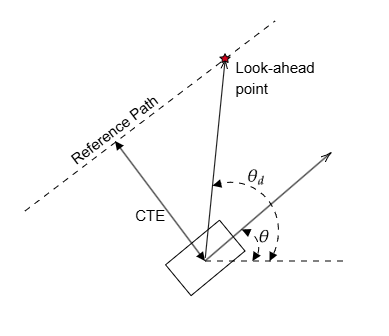
The look-ahead distance selects a point on the reference path a fixed distance ahead of the vehicle to compute the error signals, which prevents overreacting to immediate small deviations and yields smoother steering commands.

• Short look-ahead (small distance): more reactive, faster correction, can cause oscillations.

• Long look-ahead (large distance): smoother tracking, slower response to abrupt path changes.

The look-ahead parameter trades responsiveness for smoothness and is tuned with vehicle speed and path curvature in mind.

Set the manually tuned PID controller gains and look ahead distance.

gains.kp_cte = 0.15;
gains.ki_cte = 0.005;
gains.kd_cte = 0.3;
gains.kp_head = 1.5;
gains.lookahead = 5.0;

The initial state of vehicle is offset from the first way point by a fixed distance.

initial_offset = [1, -1, 0.2];
q0 = waypoints(1,:) + initial_offset;

The baseline controller has to bring the vehicle to reference path and follow it from this initial position. Run the baseline PID controller and visualize the dubins car reference path following

[states_pid,t_pid,steer_pid,cte_pid] = run_pid_sim(q0,ref_path,total_path_length,gains,v,r_min,dt);

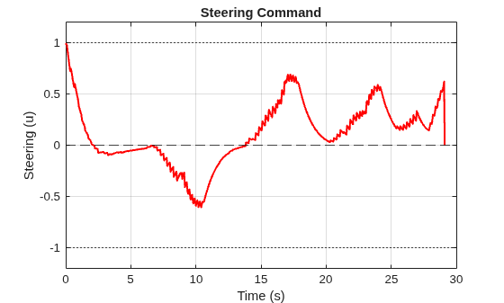
Plot the tracking trajectory with cross-track error and steering history.

plot_tracking(states_pid,t_pid,steer_pid,cte_pid,ref_path,waypoints,q0,"PID Tracking");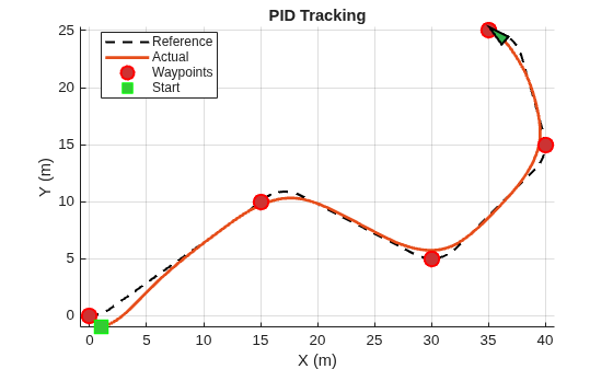

Obstacle Avoidance with Control Barrier Function

For the Dubins car model, impose a safety constraint that car should avoid collision with a circular obstacle placed at $\left[x_{obs},y_{obs}\right]=\left[15,10\right]$ with radius $$\sqrt{10}$$ m.

obs_x = 15;
obs_y = 10;
obs_r = sqrt(10);

The control barrier function for the corresponding safety constraint is mathematically defined as:

$$h\left(x,y\right)={\left(x-15\right)}^2+{\left(y-10\right)}^2-10$$

Derive the Lie derivative of CBF and form the QP problem for safe control synthesis.

The constraint equation for safe control is $\underset{}{\overset{\dot{}}{h}}\left(q,u\right)\ge -\gamma h\left(q\right)$, where $q={\left[x,y,\theta \right]}^{\prime }$ is the state vector.

Taking the first Lie derivative of the barrier function with respect to states of Dubins car,

$$\underset{}{\overset{\dot{}}{h}}\left(q,u\right)=\frac{\partial h}{\partial q}\underset{}{\overset{\dot{}}{q}}$$

$\underset{}{\overset{\dot{}}{h}}\left(q,u\right)=L_{f}h=\left[2*\left(x-x_{obs}\right),2*\left(y-y_{obs}\right),0\right]$

$\left[\begin{array}{c}\underset{}{\overset{\dot{}}{x}}\\ \underset{}{\overset{\dot{}}{y}}\\ \underset{}{\overset{\dot{}}{\theta }}\end{array}\right]$

$=2v*\left(x-x_{obs}\right)\cos \left(\theta \right)+$

$2v*\left(y-y_{obs}\right)\sin \left(\theta \right)$

The first Lie derivative does not expose the control term $u\left(t\right)$. Safety constraints require the control to appear linearly in the constraint equation. Therefore, take the second Lie derivative [3].

$\underset{}{\overset{¨}{h}}\left(q,u\right)=\frac{\partial L_{f}h}{\partial q}\underset{}{\overset{\dot{}}{q}}=\left[\begin{array}{ccc}2v*\cos \left(\theta \right)& 2v*\sin \left(\theta \right)& -2v*\left(x-x_{obs}\right)\sin \left(\theta \right)+2v*\left(y-y_{obs}\right)\cos \left(\theta \right)\end{array}\right]$

$\left[\begin{array}{c}\underset{}{\overset{\dot{}}{x}}\\ \underset{}{\overset{\dot{}}{y}}\\ \underset{}{\overset{\dot{}}{\theta }}\end{array}\right]$

The control term appears in the second lie derivative as follows:

$$\underset{}{\overset{¨}{h}}\left(q,u\right)=L_f^{2}h+L_g{L}_{f}hu=2v^2+\left(-2v*\left(x-x_{obs}\right)\sin \left(\theta \right)+2v*\left(y-y_{obs}\right)\cos \left(\theta \right)\right)\frac{v}{r_{\min }}u$$

The second-order CBF safety constraints and QP formulation for the Dubins car collision avoidance problem can be defined as:

$$\begin{array}{l}{u}^{*}=\underset{u}{\min }\frac{1}{2}{\Vert u-u_{pid}\Vert }^2\\ s.t{L}_f^{2}h+L_g{L}_{f}hu+{\gamma }_{1}h+{\gamma }_2{L}_{f}h\ge 0\end{array}$$

Control Barrier Function Setup

Below is a concise example of creating a ControlBarrierFunction object for a three-state, one-action Dubins car, configuring the number of constraints and relative order, and assigning the required function names for the barrier and Lie-derivative evaluations.

Create CBF object with number of three states, one control action, one constraint, and a relative order of two.

cbf = ControlBarrierFunction(3,1,...
    NumOfConstraints=1, ...
    RelativeOrder=2);

Assign function names for the Barrier function and Lie derivative function. These functions must be on the MATLAB path.

cbf.Constraints.BarrierFcn = "BarrierFcn";             % h(x)
cbf.Constraints.LieDerivativeFcn = "LieDerivativeFcn"; % Li_f h and Li_g Li_f h

Tuning the CBF constraint factor $\left(\gamma \right)$ and constraint power $\left(\beta \right)$ shapes how aggressively the safety constraint enforces invariance: increasing $\gamma$ generally makes the CBF act earlier and more strongly reducing allowable approach to the unsafe set, while decreasing $\gamma$ delays intervention and lets the nominal controller act longer. The $\beta$ exponent controls the nonlinearity of the penalty on the barrier terms—value 1 produce roughly linear constraints, while larger $\beta$ amplify small violations and can produce more conservative, sharper interventions.

For the Dubins car problem, set the ConstraintFactor and ConstraintPower parameters.

cbf.Constraints.ConstraintFactor = 10;
cbf.Constraints.ConstraintPower  = 1;

Run the PID+CBF safe obstacle avoidance and reference tracking control loop and return the tracking and control history for plots.

[states_cbf,t_cbf,steer_cbf,~,~] = run_pidcbf_sim( ...
    q0,ref_path,total_path_length,gains,v,r_min,dt,cbf);

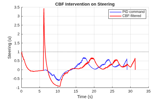
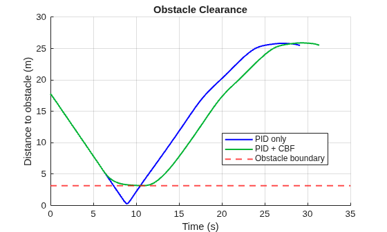
Plot the trajectory tracking and collision avoiding dubins car path with cross-track error and steering history.

plot_comparison(states_pid,t_pid,states_cbf,t_cbf, ...
    steer_cbf,steer_pid,ref_path,waypoints,obs_x,obs_y,obs_r)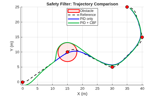

Generate Lie Derivatives

The ControlBarrierFunction object requires both a barrier function $h\left(x\right)$ and the appropriate Lie derivative functions. Hand-deriving these Lie derivatives (especially for higher relative orders or more complex barrier functions) is slow and error-prone.

The generateLieDerivativeFcn function object can auto-generate the required Lie-derivative function from a user-provided barrier function $h\left(x\right)$ and system dynamics functions.

Generate the Lie derivative function for the defined control barrier function and Dubins car dynamics.

cbf = generateLieDerivativeFcn(cbf,"DubinCarModel");

The generateLieDerivativeFcn automatically updates cbf to use the generated Lie derivative function.

Rerun the simulation with updated cbf object with auto-generated Lie derivatives and check if the results match with the hand-derived Lie derivatives

[states_cbf,t_cbf,steer_cbf,~, ~] = run_pidcbf_sim( ...
    q0,ref_path,total_path_length,gains,v,r_min,dt,cbf);

Plot the trajectory tracking and collision avoidance using PID+CBF with auto generated lie derivatives.

plot_comparison(states_pid,t_pid,states_cbf,t_cbf, ...
    steer_cbf,steer_pid,ref_path,waypoints,obs_x,obs_y,obs_r)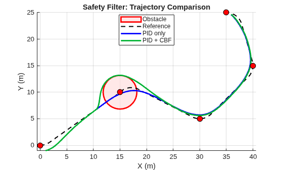

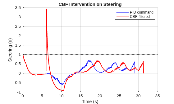
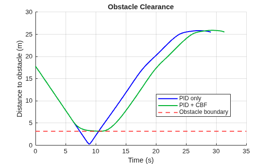
The results from the automatically generated Lie derivatives are identical to those obtained with the hand-derived Lie derivatives. This result confirms that generateLieDerivativeFcn produces mathematically equivalent expressions. The trajectory, steering commands, and obstacle clearance all match exactly between the two approaches.

Summary

This example demonstrates a programmatic workflow for using a control barrier function to enforce safety for a Dubins car while a simple PID steering controller provides nominal tracking. The example also demonstrated that a control barrier function can preserve nominal behavior away from hazards and intervenes minimally to maintain clearance, providing a modular safety layer that integrates with simple feedback controllers.

References

[1] Reeds, James, and Lawrence Shepp. "Optimal paths for a car that goes both forwards and backwards." Pacific journal of mathematics 145.2 (1990): 367-393..

[2] Ames, Aaron D., et al. "Control barrier functions: Theory and applications." 2019 18th European control conference (ECC). IEEE, 2019.

[3] W. Xiao and C. Belta, "High-Order Control Barrier Functions," in IEEE Transactions on Automatic Control, vol. 67, no. 7, pp. 3655-3662, July 2022, doi: 10.1109/TAC.2021.3105491.

Local Functions

function [states,t_vec,steering,cte] = run_pid_sim(q0,ref_path,total_path_length,gains,v,r_min,dt)
% Simulate Dubins car tracking a reference path using PID control.
% Returns state trajectory, time vector, steering commands, and cross-track error.

% Estimate simulation duration with 10% margin, then compute number of steps.
num_steps = ceil(total_path_length / v * 1.1 / dt);

% Preallocate output arrays
states = zeros(num_steps, 3);
steering = zeros(num_steps, 1);
cte = zeros(num_steps, 1);
t_vec = (0:num_steps-1)' * dt;
states(1,:) = q0;

% Initialize PID controller integrator and derivative state.
ctrl.int_cte = 0;
ctrl.prev_cte = 0;

for k = 1:(num_steps-1)
    % Compute PID steering command based on cross-track and heading errors.
    [u, ctrl, err] = pid_path_controller(states(k,:),ref_path,gains,ctrl,dt);
    steering(k) = u;
    cte(k) = err.cte;

    % Integrate Dubins car dynamics using midpoint method for heading.
    theta = states(k,3);
    theta_new = theta + (v/r_min)*u*dt;
    theta_mid = (theta + theta_new)/2;
    states(k+1,:) = [states(k,1) + v*cos(theta_mid)*dt, ...
        states(k,2) + v*sin(theta_mid)*dt, theta_new];

    % Terminate early when car reaches end of reference path.
    if norm(states(k+1,1:2) - ref_path(end,1:2)) < 1.0
        states = states(1:k+1,:);
        steering = steering(1:k+1);
        cte = cte(1:k+1);
        t_vec = t_vec(1:k+1);
        return;
    end
end
end

function [states,t_vec,steering,cte,steering_pid] = run_pidcbf_sim(q0,ref_path,total_path_length,gains,v,r_min,dt,cbf)
% Simulate Dubins car with PID tracking and CBF safety filter.
% The CBF solves a QP to minimally modify the PID command for obstacle avoidance.
% Returns state trajectory, filtered steering, cross-track error, and raw PID commands.

% Estimate simulation duration with 10% margin
num_steps = ceil(total_path_length / v * 1.1 / dt);

% Preallocate output arrays (steering_pid stores unfiltered PID commands for comparison).
states = zeros(num_steps, 3);
steering = zeros(num_steps, 1);
steering_pid = zeros(num_steps, 1);
cte = zeros(num_steps, 1);
t_vec = (0:num_steps-1)' * dt;
states(1,:) = q0;

% Initialize PID controller integrator and derivative state.
ctrl.int_cte = 0;
ctrl.prev_cte = 0;

for k = 1:(num_steps-1)
    % Compute nominal PID steering command.
    [u_pid,ctrl,err] = pid_path_controller(states(k,:),ref_path,gains,ctrl,dt);
    % Apply CBF safety filter: solve QP to find closest safe steering to u_pid
    u_star = solve(cbf,states(k,:)',u_pid,ActionMin=-1,ActionMax=1);

    steering_pid(k) = u_pid;
    steering(k) = u_star;
    cte(k) = err.cte;

    % Integrate dynamics using CBF-filtered steering (midpoint method).
    theta = states(k,3);
    theta_new = theta + (v/r_min)*u_star*dt;
    theta_mid = (theta + theta_new)/2;
    states(k+1,:) = [states(k,1) + v*cos(theta_mid)*dt, ...
        states(k,2) + v*sin(theta_mid)*dt, theta_new];

    % Terminate early when car reaches end of reference path.
    if norm(states(k+1,1:2) - ref_path(end,1:2)) < 1.0
        states = states(1:k+1,:);
        steering = steering(1:k+1);
        steering_pid = steering_pid(1:k+1);
        cte = cte(1:k+1);
        t_vec = t_vec(1:k+1);
        return;
    end
end
end