このページの内容は最新ではありません。最新版の英語を参照するには、ここをクリックします。

dtw

動的タイム ワーピングを使用した信号間の距離

構文

dist = dtw(x,y)

[dist,ix,iy] = dtw(x,y)

[___] = dtw(x,y,maxsamp)

[___] = dtw(___,metric)

dtw(___)

説明

dist = dtw(x,y) は、2 つのベクトル x と y を、対応する点間のユークリッド距離の和 dist が最小となる時点の共通セット上に引き伸ばします。入力を引き伸ばすために、dtw は x と y の各要素を必要な回数だけ繰り返します。x と y が行列の場合、dist は列の繰り返しにより引き伸ばしを行います。その場合、x と y の行数は同じでなければなりません。

[dist,ix,iy] = dtw(x,y) は、時点の共通セット、すなわち "ワーピング パス" を返し、それらの間で dist は x(ix) と y(iy) が取り得る最小のものになります。

ベクトル ix とベクトル iy は同じ長さです。それぞれに、対応する信号 x または y の要素に対するインデックスが必要な回数だけ繰り返される単調増加数列が含まれます。

x と y が行列の場合、ix と iy は x(:,ix) と y(:,iy) の分離間隔が最小限となる値になります。

[___] = dtw(x,y,maxsamp) は、ワーピング パスが x と y 間の直線近似の maxsamp サンプル内になるように制限します。この構文は、前述の構文の出力引数のいずれかを返します。

[___] = dtw(___,metric) は、前述の構文の入力引数のいずれかに加えて使用する距離計量を指定します。

出力引数を指定しない dtw(___) は、元の信号と整列後の信号をプロットします。

• 信号が実数ベクトルの場合、関数は元の 2 つの信号を 1 つのサブプロットに表示し、整列後の信号をその下のサブプロットに表示します。

• 信号が複素数ベクトルの場合、関数は元の信号と整列後の信号を 3 次元プロットに表示します。

• 信号が実数行列の場合、関数は imagesc を使用して元の信号と整列後の信号を表示します。

• 信号が複素行列の場合、関数は実数部と虚数部を各イメージの上半分と下半分にプロットします。

例

チャープおよび正弦波の動的タイム ワーピング

チャープと正弦波の 2 つの実信号を生成します。

x = cos(2*pi*(3*(1:1000)/1000).^2);
y = cos(2*pi*9*(1:399)/400);

動的タイム ワーピングを使用して、点の間のユークリッド距離の和が最小となるように信号を整列させます。整列後の信号と距離を表示します。

dtw(x,y);

正弦波周波数を初期値の 2 倍に変更します。計算を繰り返します。

y = cos(2*pi*18*(1:399)/400);

dtw(x,y);

各信号に虚数部を追加します。初期の正弦波周波数に戻します。動的タイム ワーピングを使用し、ユークリッド距離の二乗和を最小化することによって信号を整列させます。

x = exp(2i*pi*(3*(1:1000)/1000).^2);
y = exp(2i*pi*9*(1:399)/400);

dtw(x,y,'squared');

書体サンプルの位置合わせ

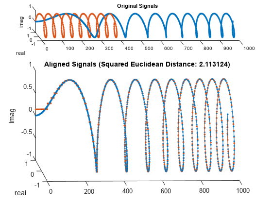
初期のコンピューターの出力に似た書体を考案します。それを使用して MATLAB® という単語を書きます。

chr = @(x)dec2bin(x')-48;

M = chr([34 34 54 42 34 34 34]);
A = chr([08 20 34 34 62 34 34]);
T = chr([62 08 08 08 08 08 08]);
L = chr([32 32 32 32 32 32 62]);
B = chr([60 34 34 60 34 34 60]);

MATLAB = [M A T L A B];

ランダムな文字の列を繰り返し、間隔を変えて単語を壊します。元の単語と 3 つの壊れたバージョンを表示します。再現可能な結果が必要な場合は、乱数発生器をリセットします。

rng('default')

c = @(x)x(:,sort([1:6 randi(6,1,3)]));

subplot(4,1,1,'XLim',[0 60])
spy(MATLAB)
xlabel('')
ylabel('Original')

for kj = 2:4
    subplot(4,1,kj,'XLim',[0 60])
    spy([c(M) c(A) c(T) c(L) c(A) c(B)])
    xlabel('')
    ylabel('Corrupted')
end

壊れたバージョンの単語をさらに 2 つ生成します。動的タイム ワーピングを使用してこの 2 つを位置合わせします。

one = [c(M) c(A) c(T) c(L) c(A) c(B)];
two = [c(M) c(A) c(T) c(L) c(A) c(B)];

[ds,ix,iy] = dtw(one,two);

onewarp = one(:,ix);
twowarp = two(:,iy);

位置合わせしていない単語と位置合わせした単語を表示します。

figure

subplot(4,1,1)
spy(one)
xlabel('')
ylabel('one')

subplot(4,1,2)
spy(two,'r')
xlabel('')
ylabel('two')

subplot(4,1,3)
spy(onewarp)
xlabel('')
ylabel('onewarp')

subplot(4,1,4)
spy(twowarp,'r')
xlabel('')
ylabel('twowarp')

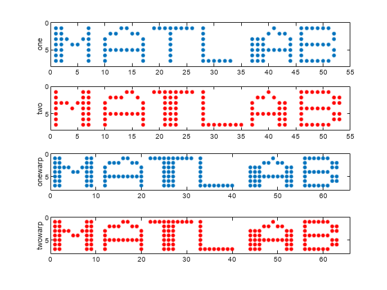
dtw の組み込み機能を使用して計算を繰り返します。

dtw(one,two);

制約付きワーピング パス

異なる長さの谷で隔てられた 2 つの明確なピークから構成される信号を 2 つ生成します。信号をプロットします。

x1 = [0 1 0 0 0 0 0 0 0 0 0 1 0]*.95;
x2 = [0 1 0 1 0]*.95;

subplot(2,1,1)
plot(x1)
xl = xlim;
subplot(2,1,2)
plot(x2)
xlim(xl)

ワーピング パスを制限せずに信号を整列させます。完全な整列を行うには、関数が、短い方の信号の 1 つのサンプルのみを反復する必要があります。

figure
dtw(x1,x2);

2 つの信号の間のワーピング パスと直線近似をプロットします。整列を達成するため、関数によってピーク間のトラフを十分に広げます。

[d,i1,i2] = dtw(x1,x2);

figure
plot(i1,i2,'o-',[i1(1) i1(end)],[i2(1) i2(end)])

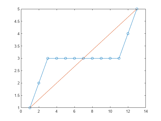
計算を繰り返しますが、今度は、ワーピング パスが最大 3 つの要素において直線近似から逸脱するように制約を付けます。引き伸ばした信号とワーピング パスをプロットします。

[dc,i1c,i2c] = dtw(x1,x2,3);

subplot(2,1,1)
plot([x1(i1c);x2(i2c)]','.-')
title(['Distance: ' num2str(dc)])
subplot(2,1,2)
plot(i1c,i2c,'o-',[i1(1) i1(end)],[i2(1) i2(end)])

制約によってワーピングがサンプルの小さなサブセットに集中しすぎることはなくなりますが、整列の質が低下します。1 サンプルの制約を付けて計算を繰り返します。

dtw(x1,x2,1);

音声信号の動的タイム ワーピング

$$F_s=7418Hz$$ でサンプリングされた音声信号を読み込みます。ファイルには、"MATLAB®" という単語を発声している女性の録音音声が含まれています。

load mtlb

% To hear, type soundsc(mtlb,Fs)

2 つの /æ/ の音素のインスタンスに対応する 2 つのセグメントを抽出します。最初のものはおおよそ 150 ms から 250 ms の間に発生し、2 番目は 370 ms から 450 ms の間に発生します。2 つの波形をプロットします。

a1 = mtlb(round(0.15*Fs):round(0.25*Fs));
a2 = mtlb(round(0.37*Fs):round(0.45*Fs));

subplot(2,1,1)
plot((0:numel(a1)-1)/Fs+0.15,a1)
title('a_1')
subplot(2,1,2)
plot((0:numel(a2)-1)/Fs+0.37,a2)
title('a_2')
xlabel('Time (seconds)')

% To hear, type soundsc(a1,Fs), pause(1), soundsc(a2,Fs)

信号間のユークリッド距離が最小となるように時間座標軸を歪めます。歪められた信号の共有の "持続時間" を計算してプロットします。

[d,i1,i2] = dtw(a1,a2);

a1w = a1(i1);
a2w = a2(i2);

t = (0:numel(i1)-1)/Fs;
duration = t(end)

duration = 0.1297

subplot(2,1,1)
plot(t,a1w)
title('a_1, Warped')
subplot(2,1,2)
plot(t,a2w)
title('a_2, Warped')
xlabel('Time (seconds)')

% To hear, type soundsc(a1w,Fs), pause(1), sound(a2w,Fs)

単語全体で実験を繰り返します。女性と男性が発声する「strong」という単語が含まれているファイルを読み込みます。この信号は 8 kHz でサンプリングされています。

load('strong.mat')

% To hear, type soundsc(her,fs), pause(2), soundsc(him,fs)

信号間の絶対距離が最小となるように時間座標軸を歪めます。元の信号と変換後の信号をプロットします。それらの歪められた共有 "持続時間" を計算します。

dtw(her,him,'absolute');
legend('her','him')

[d,iher,ihim] = dtw(her,him,'absolute');
duration = numel(iher)/fs

duration = 0.8394

% To hear, type soundsc(her(iher),fs), pause(2), soundsc(him(ihim),fs)

手書き文字の位置合わせのための動的タイム ワーピング

ファイル MATLAB1.gif と MATLAB2.gif には、"MATLAB®" という単語の 2 つの手書き文字のサンプルが含まれています。ファイルを読み込み、動的タイム ワーピングを使用して x 軸に沿ってそれらを配置します。

samp1 = 'MATLAB1.gif';
samp2 = 'MATLAB2.gif';

x = double(imread(samp1));
y = double(imread(samp2));

dtw(x,y);

入力引数

x — 入力信号

ベクトル | 行列

実数または複素数のベクトルまたは行列として指定される入力信号。

データ型: single | double
複素数のサポート: あり

y — 入力信号

ベクトル | 行列

実数または複素数のベクトルまたは行列として指定される入力信号。

データ型: single | double
複素数のサポート: あり

maxsamp — 調整ウィンドウの幅

Inf (既定値) | 正の整数

調整ウィンドウの幅。正の整数で指定します。

データ型: single | double

metric — 距離計量

'euclidean' (既定値) | 'absolute' | 'squared' | 'symmkl'

距離計量。'euclidean'、'absolute'、'squared'、または 'symmkl' で指定します。X と Y が両方とも K 次元の信号である場合、metric は X の m 番目のサンプルと Y の n 番目のサンプルの間の距離 d_mn(X,Y) を規定します。d_mn(X,Y) の詳細については、動的タイム ワーピングを参照してください。

• 'euclidean' — 距離の二乗和根。ユークリッド計量または ℓ₂ 計量とも呼ばれます。

  $$d_{mn}(X,Y)=\sqrt{{\displaystyle \sum _{k=1}^K{\left(x_{k,m}-y_{k,n}\right)}^{*}\left(x_{k,m}-y_{k,n}\right)}}$$

• 'absolute' — 差の絶対値の総和。マンハッタン計量、街区計量、タクシー計量または ℓ₁ 計量とも呼ばれます。

  $$d_{mn}(X,Y)={\displaystyle \sum _{k=1}^K\left|x_{k,m}-y_{k,n}\right|}={\displaystyle \sum _{k=1}^K\sqrt{{\left(x_{k,m}-y_{k,n}\right)}^{*}\left(x_{k,m}-y_{k,n}\right)}}$$

• 'squared' — ユークリッド計量の 2 乗。距離の二乗和で構成されます。

  $$d_{mn}(X,Y)={\displaystyle \sum _{k=1}^K{\left(x_{k,m}-y_{k,n}\right)}^{*}\left(x_{k,m}-y_{k,n}\right)}$$

• 'symmkl' — 対称カルバック・ライブラー距離。この計量は、正の実数の X と Y に対してのみ有効です。

  $$d_{mn}(X,Y)={\displaystyle \sum _{k=1}^K\left(x_{k,m}-y_{k,n}\right)\left(\log x_{k,m}-\log y_{k,n}\right)}$$

出力引数

dist — 最小距離

正の実数のスカラー

信号間の最小距離。正の実数のスカラーとして返されます。

ix — 1 番目の信号のワーピング パス

インデックスのベクトル | インデックスの行列

1 番目の信号のワーピング パス。インデックスのベクトルまたは行列として返されます。

iy — 2 番目の信号のワーピング パス

インデックスのベクトル | インデックスの行列

2 番目の信号のワーピング パス。インデックスのベクトルまたは行列として返されます。

詳細

動的タイム ワーピング

同じ順序に並んだ同等の特徴をもつ 2 つの信号が、セクションの持続時間の差によって非常に異なって見える場合があります。動的タイム ワーピングはこれらの持続時間を歪めて、対応する特徴が共通の時間軸上の同じ位置に現れるようにするため、信号間の類似点が強調されます。

次の 2 つの K 次元信号を考えます。

$$X=\left[\begin{array}{cccc}{x}_{1,1}& x_{1,2}& \cdots & x_{1,M}\\ x_{2,1}& x_{2,2}& \cdots & x_{2,M}\\ ⋮& ⋮& \ddots & ⋮\\ x_{K,1}& x_{K,2}& \cdots & x_{K,M}\end{array}\right]$$

および

$$Y=\left[\begin{array}{cccc}{y}_{1,1}& y_{1,2}& \cdots & y_{1,N}\\ y_{2,1}& y_{2,2}& \cdots & y_{2,N}\\ ⋮& ⋮& \ddots & ⋮\\ y_{K,1}& y_{K,2}& \cdots & y_{K,N}\end{array}\right],$$

これらの信号には、それぞれ M 個と N 個のサンプルがあります。metric で指定された X の m 番目のサンプルと Y の n 番目のサンプルの間の距離 d_mn(X,Y) が与えられた場合、dist は X と Y を、大域的な信号間の距離尺度が最小となるような時点の共通セット上に引き伸ばします。

最初に、この関数は d_mn(X,Y) の取りうるすべての値を次の形状のラティスに配置します。

次に、dist は、ラティス内 (これは同一長の 2 つのシーケンス ix と iy でパラメーター化されています) で以下が最小となるパスを探します。

$$d={\displaystyle \sum _{\begin{array}{c}m\in \text{ix}\\ n\in \text{iy}\end{array}}{d}_{mn}(X,Y)}$$

条件に合う dist パスとは、d₁₁(X,Y) から始まり d_MN(X,Y) で終わる、一連の "チェスのキング" の動きです。

• 垂直方向の動き: (m,n) → (m + 1,n)

• 水平方向の動き: (m,n) → (m,n + 1)

• 対角方向の動き: (m,n) → (m + 1,n + 1)

この構造では、条件に合うパスがいずれも、サンプルをスキップしたり、信号の特徴を反復したりせず、すべての信号を揃えることが確保されます。さらに、望ましいパスは、d₁₁(X,Y) と d_MN(X,Y) の間に伸びる対角方向のラインの近くを通ります。maxsamp 引数によって調整されるこの追加の制約により、ワーピングによって類似した長さのセクションが比較され、外れ値の特徴が過剰適合されることがなくなります。

以下は格子内で取りうるパスです。

次のパスは許可されていません。

信号全体が揃っていない	サンプルをスキップ	元の方向に戻り、特徴を反復

参照

[1] Paliwal, K. K., Anant Agarwal, and Sarvajit S. Sinha. "A Modification over Sakoe and Chiba’s Dynamic Time Warping Algorithm for Isolated Word Recognition." Signal Processing. Vol. 4, 1982, pp. 329–333.

[2] Sakoe, Hiroaki, and Seibi Chiba. "Dynamic Programming Algorithm Optimization for Spoken Word Recognition." IEEE^® Transactions on Acoustics, Speech, and Signal Processing. Vol. ASSP-26, No. 1, 1978, pp. 43–49.

拡張機能

C/C++ コード生成
MATLAB® Coder™ を使用して C および C++ コードを生成します。

バージョン履歴

R2016a で導入

参考

alignsignals | edr | finddelay | findsignal | xcorr