Main Content

hinfstruct

H tuning of fixed-structure controllers

Description

The hinfstruct command extends classical H synthesis (see hinfsyn) to fixed-structure control systems. If you are unfamiliar with constructing weighting functions to capture design requirements for H synthesis, use systune or looptune instead.

example

CL = hinfstruct(CL0) tunes the free parameters of the tunable genss model CL0. This tuning minimizes the H norm of the closed-loop transfer function modeled by CL0. The model CL0 represents a closed-loop control system that includes tunable components such as controllers or filters. CL0 can also include weighting functions that capture design requirements.

example

[CL,gamma,info] = hinfstruct(CL0) returns gamma (the minimum H norm) and a data structure info with additional information about each optimization run.

example

[CL,gamma,info] = hinfstruct(CL0,options) specifies additional options for the optimizer using hinfstructOptions.

[C,gamma,info] = hinfstruct(P,C0,options) tunes the parametric controller blocks C0. This tuning minimizes the H norm of the closed-loop system CL0 = lft(P,C0). To use this syntax, express your control system and design requirements as a Standard Form model, as in the following illustration.

Standard LFT structure for H-infinity synthesis. The plant, P, has inputs {w,u} and outputs {z,y}. The controller, with inputs y and outputs u, is in block-diagonal form where the diagonal elements C1, C2, …, CN are tunable.

P is a numeric LTI model that includes the fixed elements of the control architecture. P can also include weighting functions that capture design requirements. C0 can be a single tunable component (for example, a Control Design Block or a genss model) or a cell array of multiple tunable components. C is a parametric model or cell array of parametric models of the same type or types as C0.

Examples

collapse all

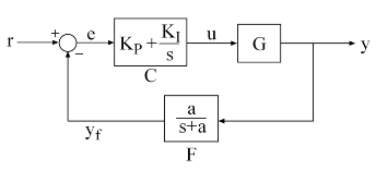
Tune the controller elements of the following control system.

The control elements are C, which is a PI controller with two free parameters, and F, which is a low-pass filter in the feedback path with one free parameter. For this example, load the plant G, a ninth-order model of the head disk assembly (HDA) in a hard disk drive.

load hinfstruct_demo G
bode(G), grid

Tune the free parameters of this control system so that the head position y tracks a step change r with a response time of about 1 ms, little or no overshoot, and no steady-state error.

First, create the tunable elements. Use a tunablePID object to parameterize the PI block, and specify the filter F0 as a transfer function depending on a tunable real parameter a.

C0 = tunablePID('C','pi');  

a = realp('a',1); 
F0 = tf(a,[1 a]);

F0 is a genss model.

Next, express the design goals as weights on the plant model, and append them to the closed-loop system. For reasons described in detail in Fixed-Structure H-infinity Synthesis with hinfstruct, the following configuration of weighting functions achieves the design requirements for this problem.

Here, LS is the desired shape of the open-loop response L(s)=F(s)G(s)C(s).

wc = 1000;  % target crossover
s = tf('s');
LS = (1+0.001*s/wc)/(0.001+s/wc);

As discussed in Fixed-Structure H-infinity Synthesis with hinfstruct, the design requirements are satisfied if the Η norm of this control structure is less than 1.

Use connect to construct a genss model representing this control structure.

% Label the block I/Os
Wn = 1/LS;  Wn.u = 'nw';  Wn.y = 'n';
We = LS;    We.u = 'e';   We.y = 'ew';
C0.u = 'e';   C0.y = 'u';
F0.u = 'yn';  F0.y = 'yf';

% Specify summing junctions
Sum1 = sumblk('e = r - yf');
Sum2 = sumblk('yn = y + n');

% Connect the blocks together
T0 = connect(G,Wn,We,C0,F0,Sum1,Sum2,{'r','nw'},{'y','ew'});

You can now use hinfstruct to find tuned values of the tunable parameters in C0 and F0 that minimize the Η norm of T0. To reduce the risk of finding local minima, run six optimizations, started from randomized initial values for C0 and F0. The RandomStart option of hinfstructOptions specifies how many additional optimizations to run beyond the default one.

rng('default')
opt = hinfstructOptions('Display','final','RandomStart',5);
T = hinfstruct(T0,opt);
Final: Peak gain = 3.88, Iterations = 67
Final: Peak gain = 596, Iterations = 199
       Some closed-loop poles are marginally stable (decay rate near 1e-07)
Final: Peak gain = 597, Iterations = 183
       Some closed-loop poles are marginally stable (decay rate near 1e-07)
Final: Peak gain = 3.88, Iterations = 66
Final: Peak gain = 1.56, Iterations = 100
Final: Peak gain = 1.56, Iterations = 99

The best closed-loop gain is about 1.56, so the constraint T<1 is nearly satisfied. The hinfstruct command returns the tuned closed-loop transfer T(s). To validate the design, plot the tuned open-loop response L = F*G*C and compare it with the target loop shape LS. To compute L, use getBlockValue to get the tuned value of C(s) and use getValue to evaluate the filter F(s) for the tuned value of a.

C = getBlockValue(T,'C');
F = getValue(F0,T.Blocks);  % Propagate tuned parameters from T to F

L = G*C*F;
bode(LS,'r--',G*C*F,'b',{1e1,1e6}), grid, 
title('Open-Loop Response'), legend('Target','Actual')

The 0 dB crossover frequency and overall loop shape are as expected. For further analysis of the result, see Fixed-Structure H-infinity Synthesis with hinfstruct.

Input Arguments

collapse all

Closed-loop system with tunable elements, specified as a genss model. This model describes the closed-loop transfer function of a control system, incorporating appropriate weighting functions on the plant inputs and outputs to capture your design requirements. For more information about selecting weights for H tuning, see Formulating Design Requirements as H-Infinity Constraints.

CL0 includes both the fixed and tunable components of the control system. You represent the tunable components of the control system using tunable control design blocks, which are stored in the CL0.Blocks property of the genss model. For more information about constructing this generalized model, see Extract Tunable Control System from Simulink Model. hinfstruct tunes the tunable elements of CL0 to minimize the H norm.

Fixed elements of the control architecture, specified as a numeric LTI model such as a state-space (ss) model. P is the plant (along with any weighting functions to capture design requirements) that results from expressing your system in standard form, pulling any tunable elements into the block-diagonal controller as shown in the following diagram.

Standard LFT structure for H-infinity synthesis. The plant, P, has inputs {w,u} and outputs {z,y}. The controller, with inputs y and outputs u, is in block-diagonal form where the diagonal elements C1, C2, …, CN are tunable.

You can obtain P in two ways:

  • In MATLAB®, model the fixed elements of your control system as numeric LTI models. Then, use block-diagram building functions (such as connect and feedback) to build P from the modeled components. Also, include any weighting functions that represent your design requirements.

  • If you have a Simulink® model of your control system and have Simulink Control Design™, use linlft (Simulink Control Design) to obtain a linear model of the fixed elements of your control system. The linlft command linearizes your Simulink model, excluding specified Simulink blocks (the blocks that represent the controller elements you want to tune). If you use weighting functions to represent your design requirements, connect them in series with the linear model of your plant to obtain P.

P can be a continuous-time or discrete-time model. In discrete time, the sample time must be specified (Ts ≠ –1), and must match the sample time of C0.

Tunable elements of the control architecture in standard form, specified as one of the following:

  • A tunable control design block such as tunableSS, tunableGain, or tunablePID

  • A generalized state-space (genss)

  • A cell array in which each entry is a tunable block or genss model

For more information and examples of creating tunable models, see Models with Tunable Coefficients.

C0 can be a continuous-time or discrete-time model, as long as the sample time matches that of P.

Algorithm options, specified as an hinfstructOptions options set. For information about available options, see hinfstructOptions.

Output Arguments

collapse all

Tuned closed-loop system, returned as a generalized state-space (genss) model. CL is the tuned version of CL0.

The hinfstruct command tunes the free parameters of CL0 to achieve a minimum H norm. CL.Blocks contains the same control design blocks as CL0.Blocks, except that in CL, the parameters have tuned values.

To access the tuned parameter values, use getValue. You can also access them directly in CL.Blocks.

Tuned controller elements, returned as a tunable control design block, a genss model, or a cell array of tunable blocks or tunable models. C is returned in the same format as C0, and contains the same tunable blocks, except that in C, the parameters have tuned values.

Best achieved H norm of the closed-loop system, returned as a positive scalar.

When you set the hinfstructOptions option RandomStarts to a nonzero value, hinfstruct performs more than one minimization run. In that case, gamma is the smallest H norm achieved over all runs.

Detailed results from each optimization run, returned as a structure, or a structure array if the hinfstructOptions option RandomStarts is nonzero. In that case, each entry in the array is the results structure for the corresponding optimization run. The fields of info are:

  • Objective — Minimum H norm value for each run. When RandomStarts = 0, Objective = gamma.

  • Iterations — Number of iterations before convergence for each run.

  • TunedBlocks — Tuned control design blocks for each run. TunedBlocks differs from C in that C contains only the result from the best run. When RandomStarts = 0, TunedBlocks = C.

Tips

  • hinfstruct is related to hinfsyn, which also uses H techniques to design a controller for a MIMO plant. However, unlike hinfstruct, hinfsyn imposes no restriction on the structure and order of the controller. For that reason, hinfsyn always returns a smaller gamma than hinfstruct. You can therefore use hinfsyn to obtain a lower bound on the best achievable performance.

  • Using hinfstruct requires some familiarity with H techniques. You must express your design requirements as frequency-weighting functions on plant inputs and outputs, as described in Formulating Design Requirements as H-Infinity Constraints. For a simpler approach to fixed-structure tuning, use systune or looptune.

Algorithms

hinfstruct uses specialized nonsmooth optimization techniques to enforce closed-loop stability and minimize the H norm as a function of the tunable parameters. These techniques are based on the work in [1].

hinfstruct computes the H norm using the algorithm of [2] and structure-preserving eigensolvers from the SLICOT library. For more information about the SLICOT library, see https://github.com/SLICOT.

References

[1] Apkarian, Pierre, and Dominikus Noll. "Nonsmooth H Synthesis." IEEE Transactions on Automatic Control, 51, no. 1 (January 2006): 71–86. https://doi.org/10.1109/TAC.2005.860290.

[2] Bruinsma, N.A., and M. Steinbuch. "A Fast Algorithm to Compute the H Norm of a Transfer Function Matrix." Systems & Control Letters, 14, no.4 (April 1990): 287–93. https://doi.org/10.1016/0167-6911(90)90049-Z.

Extended Capabilities

Version History

Introduced in R2010b