航空 LiDAR データからの個々の樹木の属性および森林のメトリクスの抽出

この例では、航空 LiDAR データから個々の樹木の属性および森林のメトリクスを抽出する方法を示します。

森林の研究とアプリケーションでは、航空レーザースキャンシステムから取得した高密度の LiDAR データをますます利用しています。このデータにより、個々の樹木の属性とより幅広い森林のメトリクスの両方を測定できます。

この例では、航空 LiDAR システムで取得された LAZ ファイルの入力点群データを使用します。最初に、点群データを地面の点と植生の点にセグメント化します。その後、植生の点を個別の樹木にセグメント化し、個々の樹木の属性を抽出します。最後に、地面の点と植生の点の両方を使用して森林のメトリクスを計算します。次の図にプロセスの概要を示します。

データの読み込みと可視化

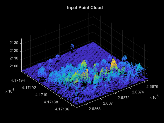
forestData.zip を一時ディレクトリに解凍し、LAZ ファイル forestData.laz から点群データを MATLAB® ワークスペースに読み込みます。データは Open Topography Dataset [1] から取得したものです。点群には主に地面と植生の点が含まれています。lasFileReaderオブジェクトのreadPointCloud関数を使用して、点群データをワークスペースに読み込みます。pcshow関数を使用して点群を可視化します。

dataFolder = fullfile(tempdir,"forestData",filesep);
dataFile = dataFolder + "forestData.laz";   
% Check whether the folder and data file already exist or not
folderExists = exist(dataFolder,"dir");
fileExists = exist(dataFile,"file");
% Create a new folder if it doesn't exist
if ~folderExists
    mkdir(dataFolder);
end
% Extract aerial data file if it doesn't exist
if ~fileExists
    unzip("forestData.zip",dataFolder);
end
% Read LAZ data from file
lasReader = lasFileReader(dataFile);
% Read point cloud along with corresponding scan angle information
[ptCloud,pointAttributes] = readPointCloud(lasReader,"Attributes","ScanAngle");
% Visualize the input point cloud
hFigInput = figure;
axInput = axes("Parent",hFigInput,"Color",[0 0 0]);
pcshow(ptCloud.Location,"Parent",axInput);
title(axInput,"Input Point Cloud");

地面のセグメント化

地面のセグメント化は、森林のメトリクスを抽出するために植生データを分離する前処理手順です。segmentGroundSMRF関数を使用して、LAZ ファイルから読み込んだデータを地面の点と地面以外の点にセグメント化します。

% Segment Ground and extract non-ground and ground points
groundPtsIdx = segmentGroundSMRF(ptCloud);
nonGroundPtCloud = select(ptCloud,~groundPtsIdx);
groundPtCloud = select(ptCloud,groundPtsIdx);
% Visualize non-ground and ground points in magenta and green, respectively
hFigSegment = figure;
axSegment = axes("Parent",hFigSegment,"Color",[0 0 0]);
pcshowpair(nonGroundPtCloud,groundPtCloud,"Parent",axSegment);
title(axSegment,"Segmented Non-Ground and Ground Points");

標高の正規化

標高を正規化することで、地形の影響を除去し、樹木の高さを正確に識別します。それらの正規化後の点を使用して樹木の属性および森林のメトリクスを計算します。標高を正規化する手順は次のとおりです。

groupsummary関数を使用して、"x" 軸および "y" 軸に沿う重複する点 (存在する場合) を除去します。
scatteredInterpolantオブジェクトを使用して内挿を作成し、点群データの各点における地面を推定します。
元の標高から、内挿した地面の標高を減算して、各点の標高を正規化します。

groundPoints = groundPtCloud.Location;
% Eliminate duplicate points along x- and y-axes
[uniqueZ,uniqueXY] = groupsummary(groundPoints(:,3),groundPoints(:,1:2),@mean);
uniqueXY = [uniqueXY{:}];
% Create interpolant and use it to estimate ground elevation at each point
F = scatteredInterpolant(double(uniqueXY),double(uniqueZ),"natural");
estElevation = F(double(ptCloud.Location(:,1)),double(ptCloud.Location(:,2)));
% Normalize elevation by ground
normalizedPoints = ptCloud.Location;
normalizedPoints(:,3) = normalizedPoints(:,3) - estElevation;
% Visualize normalized points
hFigElevation = figure;
axElevation = axes("Parent",hFigElevation,"Color",[0 0 0]);
pcshow(normalizedPoints,"Parent",axElevation);
title(axElevation,"Point Cloud with Normalized Elevation");

林冠高モデル (CHM) の生成

"林冠高モデル" (CHM) とは、地面の地形上にある樹木、建物、その他の構造物のラスター表現です。CHM を樹木の検出とセグメント化の入力として使用します。pc2dem関数を使用して、正規化後の標高値から CHM を生成します。

% Set grid size to 0.5 meters per pixel 
gridRes = 0.5;
% Generate CHM
canopyModel = pc2dem(pointCloud(normalizedPoints),gridRes,CornerFillMethod="max");
% Clip invalid and negative CHM values to zero
canopyModel(isnan(canopyModel) | canopyModel<0) = 0;
% Perform gaussian smoothing to remove noise effects
H = fspecial("gaussian",[5 5],1);
canopyModel = imfilter(canopyModel,H,"replicate","same");
% Visualize CHM
hFigCHM = figure;
axCHM = axes("Parent",hFigCHM);
imagesc(canopyModel,"Parent",axCHM);
title(axCHM,"Canopy Height Model");
axis(axCHM,"off");
colormap(axCHM,"gray");

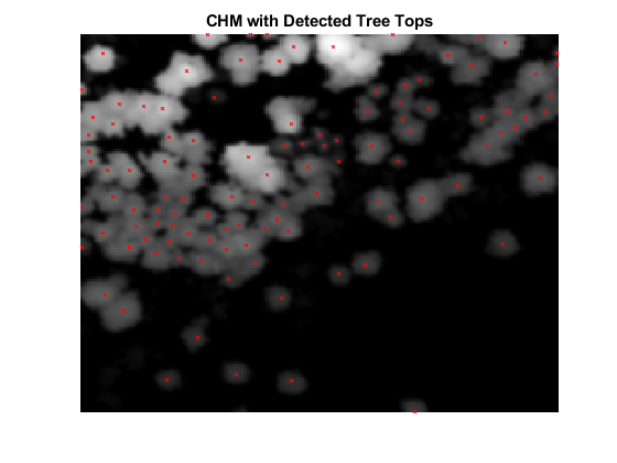
樹頂点の検出

この例にサポートファイルとして添付されている helperDetectTreeTops 補助関数を使用して、樹頂点を検出します。この補助関数は、CHM の可変ウィンドウサイズ内の局所最大値を求めることにより、樹頂点を検出します [2]。樹頂点の検出で、補助関数は正規化後の高さが minTreeHeight より大きい点のみを考慮します。

% Set minTreeHeight to 5 m 
minTreeHeight = 5;
% Detect tree tops
[treeTopRowId,treeTopColId] = helperDetectTreeTops(canopyModel,gridRes,minTreeHeight);
% Visualize treetops
hFigTreeTops = figure;
axTreeTops = axes("Parent",hFigTreeTops);
imagesc(canopyModel,"Parent",axTreeTops);
hold(axTreeTops,"on");
plot(treeTopColId,treeTopRowId,"rx","MarkerSize",3,"Parent",axTreeTops);
hold(axTreeTops,"off");
title(axTreeTops,"CHM with Detected Tree Tops");
axis(axTreeTops,"off");
colormap(axTreeTops,"gray");

個々の樹木のセグメント化

この例にサポートファイルとして添付されている helperSegmentTrees 補助関数を使用して、個々の樹木をセグメント化します。この補助関数は個々の樹木をセグメント化するために、マーカーコントロール付き watershed セグメント化 [3] を使用します。まず、この関数は樹頂点の位置を値 1 で示したバイナリマーカーイメージを作成します。次に、関数は最小値を強制配置して CHM の補数をフィルター処理することにより、樹頂点以外の最小値を除去します。次に、フィルター処理後の CHM の補数に watershed セグメント化を実行して、個々の樹木をセグメント化します。セグメント化した後、個々の樹木のセグメントを可視化します。

% Segment individual trees
label2D = helperSegmentTrees(canopyModel,treeTopRowId,treeTopColId,minTreeHeight);
% Identify row and column id of each point in label2D and transfer labels
% to each point
rowId = ceil((ptCloud.Location(:,2) - ptCloud.YLimits(1))/gridRes) + 1;
colId = ceil((ptCloud.Location(:,1) - ptCloud.XLimits(1))/gridRes) + 1;
ind = sub2ind(size(label2D),rowId,colId);
label3D = label2D(ind);
% Extract valid labels and corresponding points
validSegIds = label3D ~= 0;
ptVeg = select(ptCloud,validSegIds);
veglabel3D = label3D(validSegIds);
% Assign color to each label
numColors = max(veglabel3D);
colorMap = randi([0 255],numColors,3)/255;
labelColors = label2rgb(veglabel3D,colorMap,OutputFormat="triplets");
% Visualize tree segments
hFigTrees = figure;
axTrees = axes("Parent",hFigTrees,"Color",[0 0 0]);
pcshow(ptVeg.Location,labelColors,"Parent",axTrees);
title(axTrees,"Individual Tree Segments");
view(axTrees,2);

樹木の属性の抽出

この例にサポートファイルとして添付されている helperExtractTreeMetrics 補助関数を使用して、個々の樹木の属性を抽出します。まず、この関数は個々の樹木に属する点をラベルから特定します。次に、関数は、"x" 軸と "y" 軸に沿う樹頭の位置、樹木のおおよその高さ、樹冠の直径および面積など、樹木の属性を抽出します。補助関数は属性を table として返し、その各行は個々の樹木の属性を表します。

% Extract tree attributes
treeMetrics = helperExtractTreeMetrics(normalizedPoints,label3D);
% Display first 5 tree segments metrics
disp(head(treeMetrics,5));

    TreeId    NumPoints    TreeApexLocX    TreeApexLocY    TreeHeight    CrownDiameter    CrownArea
    ______    _________    ____________    ____________    __________    _____________    _________

      1          374        2.6867e+05      4.1719e+06       29.512          7.378          42.753 
      2           22        2.6867e+05      4.1719e+06       21.475         0.9905         0.77055 
      3          350        2.6867e+05      4.1719e+06       24.216         6.9822          38.289 
      4           53        2.6867e+05      4.1719e+06       19.509         3.1956          8.0204 
      5          117        2.6867e+05      4.1719e+06       19.399         4.0265          12.733

森林のメトリクスの抽出

この例にサポートファイルとして添付されている helperExtractForestMetrics 補助関数を使用して、正規化後の点から森林のメトリクスを抽出します。この補助関数は、まず指定された gridSize に基づくグリッドに点群を分割してから、森林のメトリクスを計算します。地形による歪みのない実際の樹木の高さに基づいて確実にメトリクスが計算されるように、地面と植生の生の点の代わりに正規化後の点を使用します。補助関数は、正規化後の高さが cutoffHeight より小さいすべての点を地面と見なし、残りの点を植生と見なします。以下の森林のメトリクスを計算します。

林冠被覆率 (CC) — "林冠被覆率" [4] とは、樹冠の垂直投影によって覆われる森林の割合です。これは、リターン総数に対する植生リターン数の割合として計算します。
ギャップ率 (GF) — "ギャップ率" [5] とは、光線が群葉やその他の樹木要素に当たらずに林冠を通過する確率です。これは、リターン総数に対する地面リターン数の割合として計算します。
葉面積指数 (LAI) — "葉面積指数" [5] とは、単位面積の地面あたりの葉面積 (片側) の量です。LAI の値を計算するには、式 $LAI = - \frac{\cos (ang) * \ln (GF)}{k}$ を使用します。ここで、ang は平均スキャン角度、GF はギャップ率です。k は吸光係数で、葉傾斜角の分布と密接に関連しています。

% Set grid size to 10 meters per pixel and cutOffHeight to 2 meters
gridSize = 10;
cutOffHeight = 2;
leafAngDistribution = 0.5;
% Extract forest metrics
[canopyCover,gapFraction,leafAreaIndex] = helperExtractForestMetrics(normalizedPoints, ...
    pointAttributes.ScanAngle,gridSize,cutOffHeight,leafAngDistribution);
% Visualize forest metrics
hForestMetrics = figure;
axCC = subplot(2,2,1,"Parent",hForestMetrics);
axCC.Position = [0.05 0.51 0.4 0.4];
imagesc(canopyCover,"Parent",axCC);
title(axCC,"Canopy Cover");
axis(axCC,"off");
colormap(axCC,"gray");
axGF = subplot(2,2,2,"Parent",hForestMetrics);
axGF.Position = [0.55 0.51 0.4 0.4];
imagesc(gapFraction,"Parent",axGF);
title(axGF,"Gap Fraction");
axis(axGF,"off");
colormap(axGF,"gray");
axLAI = subplot(2,2,[3 4],"Parent",hForestMetrics);
axLAI.Position = [0.3 0.02 0.4 0.4];
imagesc(leafAreaIndex,"Parent",axLAI);
title(axLAI,"Leaf Area Index");
axis(axLAI,"off");
colormap(axLAI,"gray");

参考文献

[1] Thompson, S. Illilouette Creek Basin Lidar Survey, Yosemite Valley, CA 2018. National Center for Airborne Laser Mapping (NCALM). Distributed by OpenTopography. https://doi.org/10.5069/G96M351N. Accessed: 2021-05-14

[2] Pitkänen, J., M. Maltamo, J. Hyyppä, and X. Yu. "Adaptive Methods for Individual Tree Detection on Airborne Laser Based Canopy Height Model." International Archives of Photogrammetry, Remote Sensing and Spatial Information Sciences 36, no. 8 (January 2004): 187–91.

[3] Chen, Qi, Dennis Baldocchi, Peng Gong, and Maggi Kelly. “Isolating Individual Trees in a Savanna Woodland Using Small Footprint Lidar Data.”Photogrammetric Engineering & Remote Sensing 72, no. 8 (August 1, 2006): 923–32. https://doi.org/10.14358/PERS.72.8.923.

[4] Ma, Qin, Yanjun Su, and Qinghua Guo. "Comparison of Canopy Cover Estimations From Airborne LiDAR, Aerial Imagery, and Satellite Imagery." IEEE Journal of Selected Topics in Applied Earth Observations and Remote Sensing 10, no. 9 (September 2017): 4225–36. https://doi.org/10.1109/JSTARS.2017.2711482.

[5] Richardson, Jeffrey J., L. Monika Moskal, and Soo-Hyung Kim. "Modeling Approaches to Estimate Effective Leaf Area Index from Aerial Discrete-Return LIDAR." Agricultural and Forest Meteorology 149, no. 6–7 (June 2009): 1152–60. https://doi.org/10.1016/j.agrformet.2009.02.007.

参考

lasFileReader | readPointCloud | segmentGroundSMRF | lidarPointAttributes