スペクトル シグネチャ マッチングを使用したターゲットの検出
この例では、スペクトル マッチング法を使用して、ハイパースペクトル イメージ内の既知のターゲットを検出する方法を示します。ハイパースペクトル イメージ内のターゲットの検出と位置特定には、既知のターゲット物質のピュア スペクトル シグネチャを使用します。この例では、スペクトル角マッパー (SAM) スペクトル マッチング法を使用して、ハイパースペクトル イメージ内の人工の屋根材 (既知のターゲット) を検出します。屋根材のピュア スペクトル シグネチャを ECOSTRESS スペクトル ライブラリから読み取り、スペクトル マッチング用の基準スペクトルとして使用します。データ キューブ内のすべてのピクセルのスペクトル シグネチャを基準スペクトルと比較し、最適に一致するピクセルのスペクトルをターゲット物質に属するものとして分類します。
この例には、Hyperspectral Imaging Library for Image Processing Toolbox™ が必要です。Hyperspectral Imaging Library for Image Processing Toolbox は、アドオン エクスプローラーからインストールできます。アドオンのインストールの詳細については、アドオンの取得と管理を参照してください。Hyperspectral Imaging Library for Image Processing Toolbox は、MATLAB® Online™ および MATLAB® Mobile™ でサポートされないため、デスクトップの MATLAB® が必要です。
この例では、パヴィア大学のデータセットから取得したデータ サンプルをテスト データとして使用します。このデータセットには、9 つのグラウンド トゥルース クラスのエンドメンバー シグネチャが格納されており、各シグネチャは長さ 103 のベクトルです。グラウンド トゥルース クラスには、アスファルト、牧草地、砂利、樹木、塗装済み金属シート、露出土壌、瀝青、セルフ ブロック レンガ、影が含まれます。これらのクラスのうち、塗装済み金属シートは通常、屋根材のタイプに属し、位置特定の対象となるターゲットです。
テスト データの読み取り
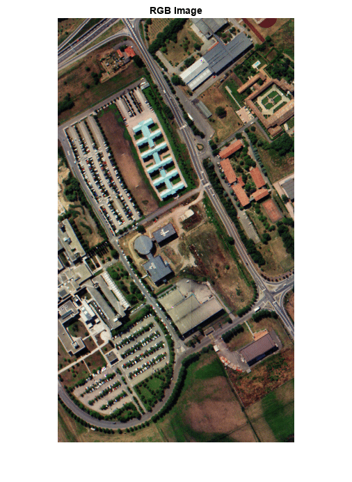
パヴィア大学のデータセットからテスト データを読み取り、このテスト データから読み取ったデータ キューブとメタデータ情報をhypercubeオブジェクトとして保存します。テスト データには、103 個のスペクトル バンドと、430 nm ~ 860 nm の範囲の波長が含まれています。幾何学的分解能は 1.3 メートル、各バンド イメージの空間分解能は 610 x 340 です。
hcube = imhypercube("paviaU.hdr");関数colorizeを使用してデータ キューブから RGB カラー イメージを推定します。RGB カラー イメージのコントラストを改善するために、ContrastStretching パラメーター値を true に設定します。RGB イメージを表示します。
rgbImg = colorize(hcube,Method="rgb",ContrastStretching=true);
imshow(rgbImg)
title("RGB Image")
基準スペクトルの読み取り
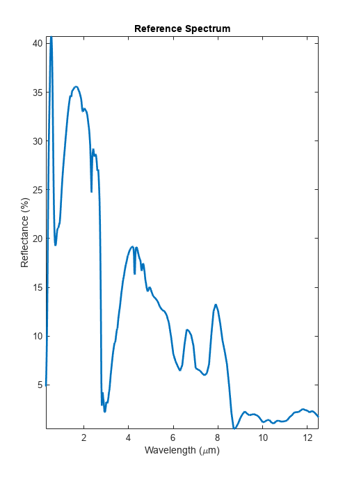
関数readEcostressSigを使用して、ECOSTRESS スペクトル ライブラリから屋根材に該当するスペクトル情報を読み取ります。
lib = readEcostressSig("manmade.roofingmaterial.metal.solid.all.0692uuucop.jhu.becknic.spectrum.txt");ECOSTRESS ライブラリから読み取った基準スペクトルのプロパティを検査します。出力構造体 lib はメタデータおよび ECOSTRESS ライブラリから読み取ったデータ値を格納します。
lib
lib = struct with fields:
                     Name: "Copper Metal"
                     Type: "manmade"
                    Class: "Roofing Material"
                 SubClass: "Metal"
             ParticleSize: "Solid"
                    Genus: [0×0 string]
                  Species: [0×0 string]
                 SampleNo: "0692UUUCOP"
                    Owner: "National Photographic Interpretation Center"
          WavelengthRange: "All"
                   Origin: "Spectra obtained from the Noncoventional Exploitation FactorsData System of the National Photographic Interpretation Center."
           CollectionDate: "N/A"
              Description: "Extremely weathered bare copper metal from government building roof flashing. Original ASTER Spectral Library name was jhu.becknic.manmade.roofing.metal.solid.0692uuu.spectrum.txt"
              Measurement: "Directional (10 Degree) Hemispherical Reflectance"
              FirstColumn: "X"
             SecondColumn: "Y"
           WavelengthUnit: "micrometer"
                 DataUnit: "Reflectance (percent)"
              FirstXValue: "0.3000"
               LastXValue: "12.5000"
          NumberOfXValues: "536"
    AdditionalInformation: "none"
               Wavelength: [536×1 double]
              Reflectance: [536×1 double]
lib に格納された波長と反射率値を読み取ります。波長と反射率のペアは、基準スペクトルまたは基準スペクトル シグネチャを構成します。
wavelength = lib.Wavelength;
reflectance = lib.Reflectance;
ECOSTRESS ライブラリから読み取った基準スペクトルをプロットします。
plot(wavelength,reflectance,LineWidth=2)
axis tight
xlabel("Wavelength (\mum)")
ylabel("Reflectance (%)")
title("Reference Spectrum")
スペクトル マッチングの実行
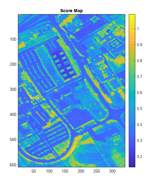
関数spectralMatchを使用して、基準スペクトルとデータ キューブの間のスペクトル類似度を求めます。既定の設定では、この関数はスペクトル角マッパー (SAM) 法を使用してスペクトルの一致を求めます。出力は、各ピクセル スペクトルと基準スペクトルのマッチングを示すスコア マップです。したがって、スコア マップはテスト データの空間次元と同じ空間次元の行列となります。この場合、スコア マップのサイズは 610 x 340 です。SAM はゲイン ファクターの影響を受けないため、地理的な照明効果により元々未知のゲイン ファクターを持つピクセル スペクトルのマッチングに使用できます。
scoreMap = spectralMatch(lib,hcube);
スコア マップを表示します。
figure(Position=[0 0 500 600])
imagesc(scoreMap)
colormap parula
colorbar
title("Score Map")
ターゲットの分類と検出
SAM スコアの一般的な値は、[0, 3.142] の範囲内にあり、測定単位はラジアンです。SAM スコアの値が低いほど、ピクセル スペクトルと基準スペクトルのマッチングが良好であることを表しています。しきい値処理方法を使用して、入力データ内のターゲット領域を空間的に局所化します。しきい値を決定するには、スコア マップのヒストグラムを検査します。発生回数が顕著な SAM スコアの最小値を使用すると、ターゲット領域を検出するためのしきい値を選択できます。
figure
imhist(scoreMap);
title("Histogram Plot of Score Map")
xlabel("Score Map Values")
ylabel("Number of Occurrences")
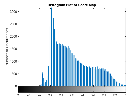
ヒストグラムのプロットから、発生回数が顕著なスコア最小値はおよそ 0.22 と推定します。このため、局所的最大値付近の値をしきい値として設定できます。この例の場合は、ターゲットを検出するためのしきい値には 0.25 を選択できます。最大しきい値より小さいピクセル値はターゲット領域として分類されます。
maxthreshold = 0.25;
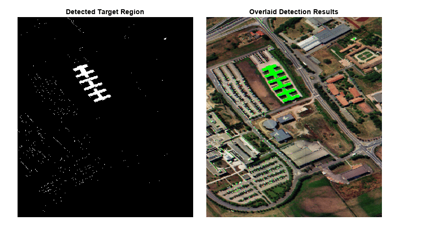
しきい値処理を実行して、スペクトル類似度が最大となるターゲット領域を検出します。ハイパースペクトル データの RGB イメージにしきい値処理されたイメージを重ね合わせます。
thresholdedImg = scoreMap <= maxthreshold;
overlaidImg = imoverlay(rgbImg,thresholdedImg,"green");
結果を表示します。
fig = figure(Position=[0 0 900 500]);
axes1 = axes(Parent=fig,Position=[0.04 0.11 0.4 0.82]);
imagesc(thresholdedImg,Parent=axes1);
colormap([0 0 0;1 1 1])
title("Detected Target Region")
axis off
axes2 = axes(Parent=fig,Position=[0.47 0.11 0.4 0.82]);
imagesc(overlaidImg,Parent=axes2)
axis off
title("Overlaid Detection Results")
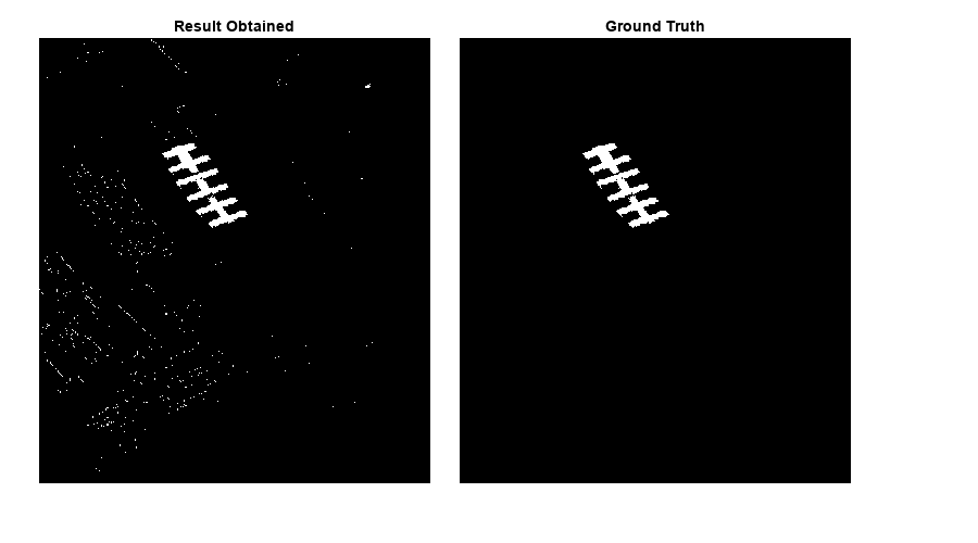
検出結果の検証
パヴィア大学のデータセットから取得したグラウンド トゥルース データを使用して、得られたターゲット検出結果を検証できます。
グラウンド トゥルース データを含む MAT ファイルを読み込みます。結果を定量的に検証するには、グラウンド トゥルースと出力の平均二乗誤差を計算します。得られた結果がグラウンド トゥルースに近い場合、この誤差は小さくなります。
load("paviauRoofingGT.mat");
err = immse(im2double(paviauRoofingGT), im2double(thresholdedImg));
disp("The mean squared error is "+err)
The mean squared error is 0.004026
fig = figure(Position=[0 0 900 500]);
axes1 = axes(Parent=fig,Position=[0.04 0.11 0.4 0.82]);
imagesc(thresholdedImg,Parent=axes1);
colormap([0 0 0;1 1 1]);
title("Result Obtained")
axis off
axes2 = axes(Parent=fig,Position=[0.47 0.11 0.4 0.82]);
imagesc(paviauRoofingGT,Parent=axes2)
colormap([0 0 0;1 1 1]);
axis off
title("Ground Truth")
参考文献
[1] Kruse, F.A., A.B. Lefkoff, J.W. Boardman, K.B. Heidebrecht, A.T. Shapiro, P.J. Barloon, and A.F.H. Goetz. "The Spectral Image Processing System (SIPS)—Interactive Visualization and Analysis of Imaging Spectrometer Data." Remote Sensing of Environment 44, no. 2–3 (May 1993): 145–63. https://doi.org/10.1016/0034-4257(93)90013-N.
[2] Chein-I Chang. "An Information-Theoretic Approach to Spectral Variability, Similarity, and Discrimination for Hyperspectral Image Analysis." IEEE Transactions on Information Theory 46, no. 5 (August 2000): 1927–32. https://doi.org/10.1109/18.857802.
[3] ECOSTRESS Spectral Library: https://speclib.jpl.nasa.gov
[4] Meerdink, Susan K., Simon J. Hook, Dar A. Roberts, and Elsa A. Abbott. “The ECOSTRESS Spectral Library Version 1.0.” Remote Sensing of Environment 230 (September 2019): 111196. https://doi.org/10.1016/j.rse.2019.05.015.
[5] Baldridge, A.M., S.J. Hook, C.I. Grove, and G. Rivera. “The ASTER Spectral Library Version 2.0.” Remote Sensing of Environment 113, no. 4 (April 2009): 711–15. https://doi.org/10.1016/j.rse.2008.11.007.
参考
hypercube | colorize | readEcostressSig | resampleSignature | removeContinuum | spectralMatch | detectTarget