Implement Digital Upconverter for FPGA
This example shows how to design a digital upconverter (DUC) for radio communication applications such as LTE, and generate HDL code.
Introduction
DUCs are widely used in digital communication transmitters to convert baseband signals to radio frequency (RF) or intermediate frequency (IF) signals. The DUC operation increases the sample rate of the signal and shifts it to a higher frequency to facilitate subsequent processing stages. The DUC in this example performs sample rate conversion using a four-stage filter chain followed by complex frequency translation.
For an example of the corresponding digital downconverter (DDC) operation, see Implement Digital Downconverter for FPGA.
The example starts by designing the DUC with DSP System Toolbox™ functions in floating point. Then, each stage is converted to fixed point, and used in a Simulink® model that generates synthesizable HDL code. The example uses these two test signals to demonstrate and verify the DUC operation:
A sinusoid that is modulated onto a 32 MHz IF carrier.
An LTE downlink signal with a bandwidth of 1.4 MHz, modulated onto a 32 MHz IF carrier.
The example downconverts the outputs of the floating-point and fixed-point DUCs, and compares the signal quality of the two outputs.
Finally, the example presents an implementation of the filter chain for FPGAs, and synthesis results.
This example uses DUCTestUtils, a helper class that contains functions for generating stimulus and analyzing the DUC output. For more information, see the DUCTestUtils.m file.
DUC Structure
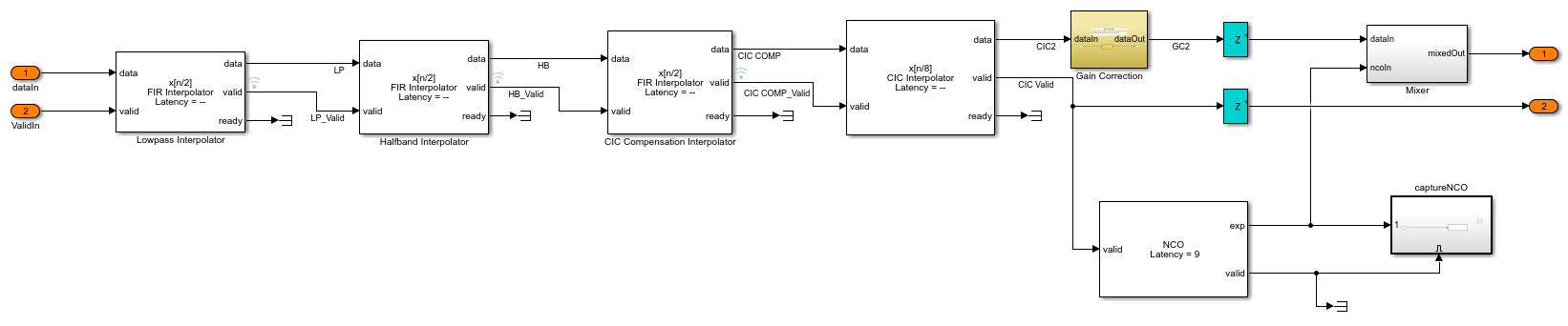
The DUC consists of an interpolating filter chain, numerically controlled oscillator (NCO), and mixer. The filter chain consists of a lowpass interpolator, halfband interpolator, CIC compensation interpolator (FIR), CIC interpolator, and CIC gain correction.
The overall response of the filter chain is equivalent to that of a single interpolation filter with the same specification. However, splitting the filter into multiple interpolation stages results in a more efficient design that uses fewer hardware resources.
The first lowpass interpolator implements the precise Fpass and Fstop characteristics of the DUC. The halfband filter is an intermediate interpolator. The lower sampling rates at the beginning of the chain mean the earlier filters can optimize resource use by sharing multipliers. The CIC compensation interpolator improves the spectral response by compensating for the later CIC droop while interpolating by two. The CIC interpolator provides a large interpolation factor, which meets the filter chain upsampling requirements.
This figure shows a block diagram of the DUC.
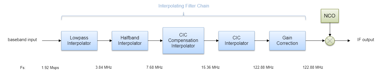
The sample rate of the input to the DUC is 1.92 Msps, and the output sample rate is 122.88 Msps. These rates give an overall interpolation factor of 64. LTE receivers use 1.92 Msps as the typical sampling rate for cell search and master information block (MIB) recovery. The DUC filters are designed to suit this application. The DUC is optimized to run at a clock rate of 122.88 MHz.
DUC Design
This section explains how to design the DUC using floating-point operations and filter-design functions in MATLAB®. The DUC object enables you to specify several characteristics that define the response of the cascade for the four filters, including passband and stopband frequencies, passband ripple, and stopband attenuation.
DUC Parameters
This example designs the DUC filter characteristics to meet these desired response values for the given input sampling rate and carrier frequency.
FsIn = 1.92e6;      % Sampling rate at input to DUC
FsOut = 122.88;     % Sampling rate at the output
Fc = 32e6;          % Carrier frequency
Fpass = 540e3;      % Passband frequency, equivalent to 36*15kHz LTE subcarriers
Fstop = 700e3;      % Stopband frequency
Ap = 0.1;           % Passband ripple
Ast = 60;           % Stopband attenuation
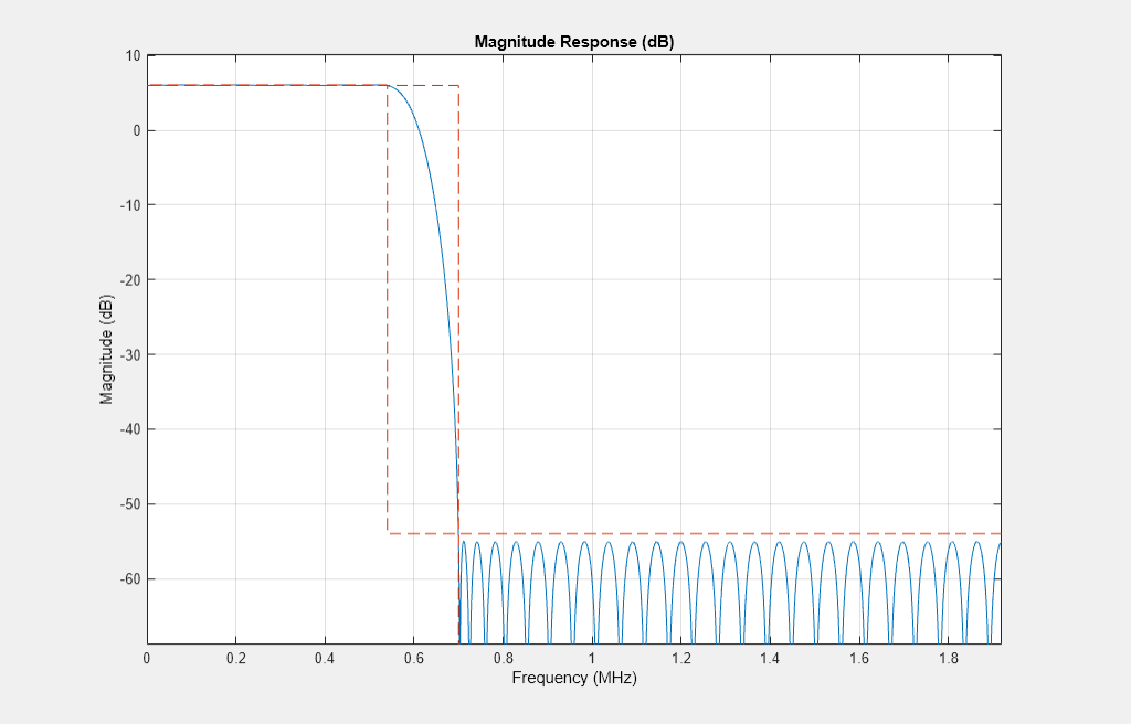
First Lowpass Interpolator
This filter interpolates by two, and operates at the lowest sampling rate of the filter chain. The low sample rate means this filter can use resource sharing for an efficient hardware implementation.
lowpassParams.FsIn = FsIn;
lowpassParams.InterpolationFactor = 2;
lowpassParams.FsOut = FsIn*lowpassParams.InterpolationFactor;

lowpassSpec = fdesign.interpolator(lowpassParams.InterpolationFactor, ...
    'lowpass','Fp,Fst,Ap,Ast',Fpass,Fstop,Ap,Ast,lowpassParams.FsOut);
lowpassFilt = design(lowpassSpec,'SystemObject',true)
lowpassFilt =

  dsp.FIRInterpolator with properties:

    InterpolationFactor: 2
        NumeratorSource: 'Property'
              Numerator: [0.0020 0.0021 4.9115e-04 -0.0027 … ] (1×69 double)

  Use get to show all properties
Display the magnitude response of the lowpass filter without gain correction.
ducPlots.lowpass = filterAnalyzer(lowpassFilt,SampleRates=FsIn*2);
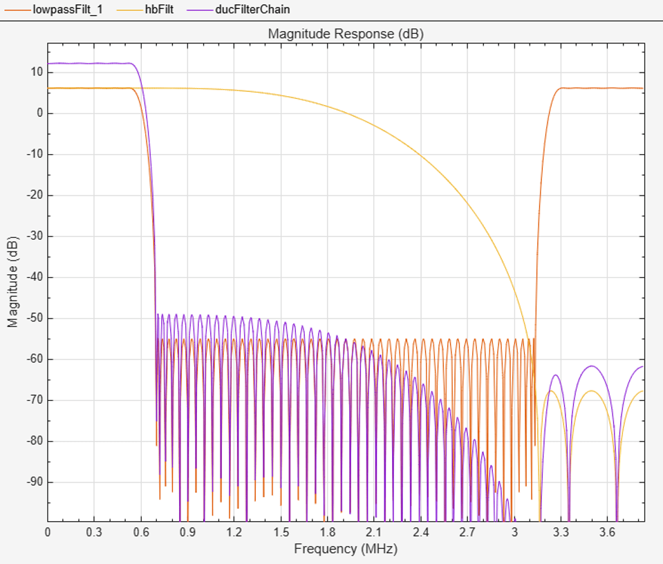
Second Halfband Interpolator
The halfband filter provides efficient interpolation by two. Halfband filters are efficient for hardware because approximately half of their coefficients are equal to zero, and those multipliers are excluded from the hardware implementation.
 hbParams.FsIn = lowpassParams.FsOut;
 hbParams.InterpolationFactor = 2;
 hbParams.FsOut = lowpassParams.FsOut*hbParams.InterpolationFactor;
 hbParams.TransitionWidth = hbParams.FsIn - 2*Fstop;
 hbParams.StopbandAttenuation = Ast;

 hbSpec = fdesign.interpolator(hbParams.InterpolationFactor,'halfband', ...
          'TW,Ast', ...
          hbParams.TransitionWidth, ...
          hbParams.StopbandAttenuation, ...
          hbParams.FsOut);

hbFilt = design(hbSpec,'SystemObject',true)
hbFilt =

  dsp.FIRInterpolator with properties:

    InterpolationFactor: 2
        NumeratorSource: 'Property'
              Numerator: [0.0178 0 -0.1129 0 0.5953 1 0.5953 … ] (1×11 double)

  Use get to show all properties
Visualize the magnitude response of the halfband interpolation.
ducFilterChain = dsp.FilterCascade(lowpassFilt,hbFilt);
ducPlots.hbFilt = filterAnalyzer(lowpassFilt,hbFilt,ducFilterChain, ...
    SampleRates=[FsIn*2,FsIn*4,FsIn*4]);
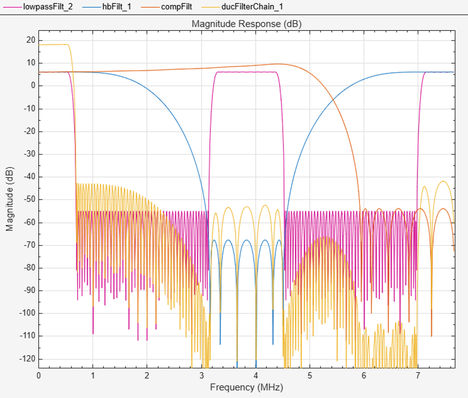
CIC Compensation Interpolator
Because the magnitude response of the last CIC filter has a significant droop within the passband region, the example uses an FIR-based droop compensation filter to flatten the passband response. The droop compensator has the same properties as the CIC interpolator. This filter implements interpolation by a factor of two, so you must also specify bandlimiting characteristics for the filter. Also, specify the CIC interpolator properties that are used for this compensation filter as well as the later CIC interpolator.
Use the design function to return a filter System object with the specified characteristics.
compParams.FsIn = hbParams.FsOut;
compParams.InterpolationFactor = 2;                                 % CIC compensation interpolation factor
compParams.FsOut = compParams.FsIn*compParams.InterpolationFactor;  % New sampling rate
compParams.Fpass = 1/2*compParams.FsIn + Fpass;                     % CIC compensation passband frequency
compParams.Fstop = 1/2*compParams.FsIn + 1/4*compParams.FsIn;       % CIC compensation stopband frequency
compParams.Ap = Ap;                                                 % Same passband ripple as overall filter
compParams.Ast = Ast;                                               % Same stopband attenuation as overall filter
N = 31;                                                             % 32 tap filter to take advantage of 16 cycles between input

cicParams.InterpolationFactor = 8;  % CIC interpolation factor
cicParams.DifferentialDelay = 1;    % CIC interpolator differential delay
cicParams.NumSections = 3;          % CIC interpolator number of integrator and comb sections

compSpec = fdesign.interpolator(compParams.InterpolationFactor,'ciccomp', ...
           cicParams.DifferentialDelay, ...
           cicParams.NumSections, ...
           cicParams.InterpolationFactor, ...
           'N,Fp,Ap,Ast', ...
           N,compParams.Fpass,compParams.Ap,compParams.Ast, ...
           compParams.FsOut);
compFilt = design(compSpec,'SystemObject',true)
compFilt =

  dsp.FIRInterpolator with properties:

    InterpolationFactor: 2
        NumeratorSource: 'Property'
              Numerator: [-6.9876e-04 -0.0099 0.0038 0.0134 … ] (1×32 double)

  Use get to show all properties
Plot the response of the CIC compensation interpolator.
ducFilterChain = dsp.FilterCascade(lowpassFilt,hbFilt,compFilt);
ducPlots.cicComp = filterAnalyzer(lowpassFilt,hbFilt,compFilt,ducFilterChain, ...
                           SampleRates=[FsIn*2,FsIn*4,FsIn*8,FsIn*8]);
CIC Interpolator
The last filter stage is implemented as a CIC interpolator because of this type of filter's ability to efficiently implement a large decimation factor. The response of a CIC filter is similar to a cascade of moving average filters, but a CIC filter uses no multiplication or division. As a result, the CIC filter has a large DC gain.
cicParams.FsIn = compParams.FsOut;
cicParams.FsOut = cicParams.FsIn*cicParams.InterpolationFactor;

cicFilt = dsp.CICInterpolator(cicParams.InterpolationFactor, ...
          cicParams.DifferentialDelay,cicParams.NumSections)
cicFilt =

  dsp.CICInterpolator with properties:

    InterpolationFactor: 8
      DifferentialDelay: 1
            NumSections: 3
     FixedPointDataType: 'Full precision'
Visualize the magnitude response of the CIC interpolation. CIC filters use fixed-point arithmetic internally, so filterAnalyzer plots both the quantized and unquantized responses.
ducFilterChain = dsp.FilterCascade(lowpassFilt,hbFilt,compFilt,cicFilt);
ducPlots.cicInter = filterAnalyzer(lowpassFilt,hbFilt,compFilt,cicFilt,ducFilterChain, ...
                      SampleRates=[FsIn*2,FsIn*4,FsIn*8,FsIn*64,FsIn*64]);

Every interpolator has a DC gain that is determined by its interpolation factor. The CIC interpolator has a larger gain than other filters. Call the gain function to get the gain factor of this filter.
Because the CIC gain is a power of two, a hardware implementation can easily correct for the gain factor by using a shift operation. For analysis purposes, the example represents the gain correction by using a one-tap dsp.FIRFilter System object. Combine the filter chain and the gain correction filter into a dsp.FilterCascade System object.
cicGain = gain(cicFilt)
Gain = lowpassParams.InterpolationFactor* ...
    hbParams.InterpolationFactor*compParams.InterpolationFactor* ...
    cicParams.InterpolationFactor*cicGain;
GainCorr = dsp.FIRFilter('Numerator',1/Gain)
cicGain =

    64


GainCorr =

  dsp.FIRFilter with properties:

            Structure: 'Direct form'
      NumeratorSource: 'Property'
            Numerator: 2.4414e-04
    InitialConditions: 0

  Use get to show all properties
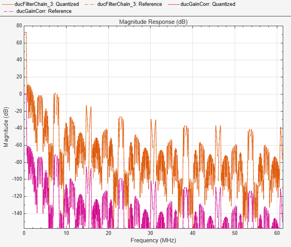
Plot the overall chain response with and without gain correction.
ducGainCorr = dsp.FilterCascade(ducFilterChain,GainCorr);
ducPlots.overallResponse = filterAnalyzer(ducFilterChain, ducGainCorr, ...
    SampleRates=[FsIn*64,FsIn*64]);
Fixed-Point Conversion
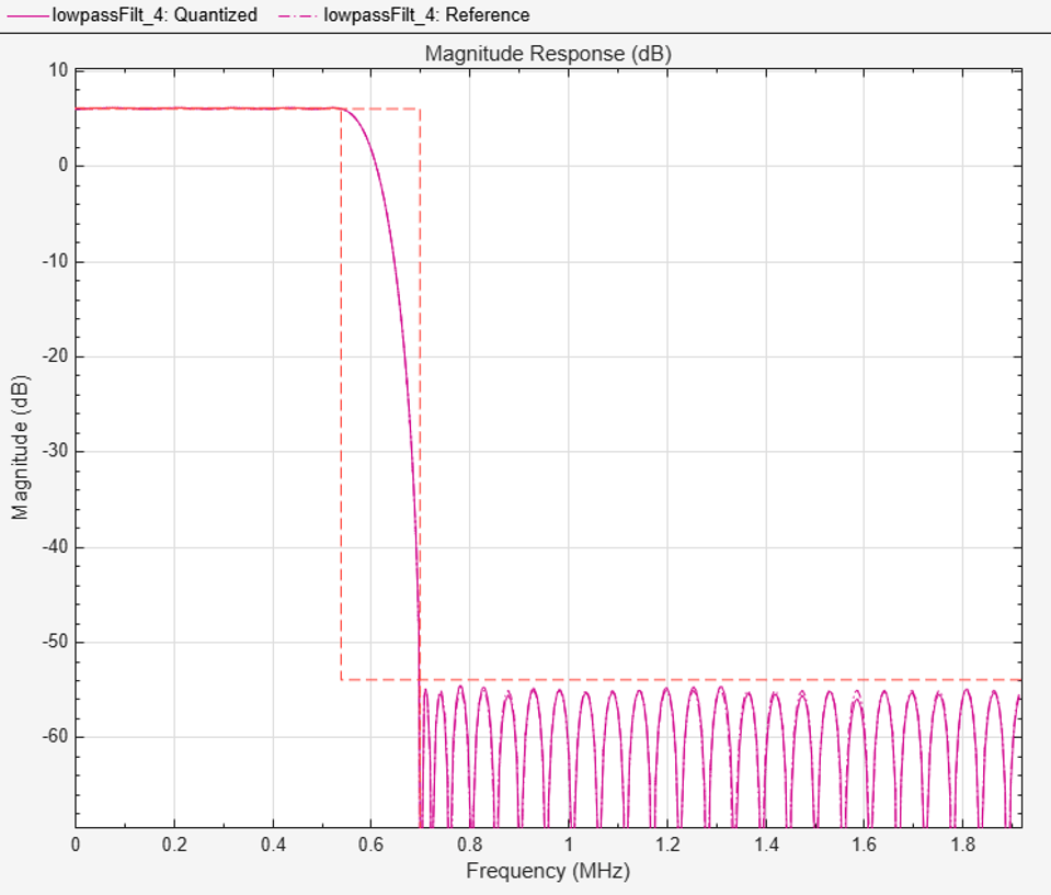
The frequency response of the floating-point DUC filter chain now meets the specification. Next, quantize each filter stage to use fixed-point types and analyze them to confirm that the filter chain still meets the specification.
Filter Quantization
This example uses 16-bit coefficients, which are sufficient to meet the specification. Using fewer than 18 bits for the coefficients minimizes the number of DSP blocks that are required for an FPGA implementation. The input to the DUC filter chain is 16-bit data with 15 fractional bits. The filter outputs are 18-bit values, which provide extra headroom and precision in the intermediate signals.
% First Lowpass Interpolator
lowpassFilt.FullPrecisionOverride = false;
lowpassFilt.CoefficientsDataType = 'Custom';
lowpassFilt.CustomCoefficientsDataType = numerictype([],16,15);
lowpassFilt.ProductDataType = 'Full precision';
lowpassFilt.AccumulatorDataType = 'Full precision';
lowpassFilt.OutputDataType = 'Custom';
lowpassFilt.CustomOutputDataType = numerictype([],18,14);

% Halfband
hbFilt.FullPrecisionOverride = false;
hbFilt.CoefficientsDataType = 'Custom';
hbFilt.CustomCoefficientsDataType = numerictype([],16,14);
hbFilt.ProductDataType = 'Full precision';
hbFilt.AccumulatorDataType = 'Full precision';
hbFilt.OutputDataType = 'Custom';
hbFilt.CustomOutputDataType = numerictype([],18,14);

% CIC Compensation Interpolator
compFilt.FullPrecisionOverride = false;
compFilt.CoefficientsDataType = 'Custom';
compFilt.CustomCoefficientsDataType = numerictype([],16,14);
compFilt.ProductDataType = 'Full precision';
compFilt.AccumulatorDataType = 'Full precision';
compFilt.OutputDataType = 'Custom';
compFilt.CustomOutputDataType = numerictype([],18,14);
For the CIC interpolator, choosing the 'Minimum section word lengths' fixed-point data type option automatically optimizes the internal wordlengths based on the output wordlength and other CIC parameters.
cicFilt.FixedPointDataType = 'Minimum section word lengths';
cicFilt.OutputWordLength = 18;
Configure the fixed-point properties of the gain correction and FIR-based System objects. The object uses the default RoundingMethod and OverflowAction property values ('Floor' and 'Wrap' respectively).
% CIC Gain Correction
GainCorr.FullPrecisionOverride = false;
GainCorr.CoefficientsDataType = 'Custom';
GainCorr.CustomCoefficientsDataType = numerictype(fi(GainCorr.Numerator,1,16));
GainCorr.OutputDataType = 'Custom';
GainCorr.CustomOutputDataType = numerictype(1,18,14);
Fixed-Point Analysis
Inspect the quantization effects with filterAnalyzer. You can analyze the filters individually or in a cascade. filterAnalyzer shows the quantized and unquantized (reference) responses overlayed. For example, this figure shows the effect of quantizing the first FIR filter stage.
ducPlots.quantizedFIR = filterAnalyzer(lowpassFilt, ...
    SampleRates=lowpassParams.FsIn*2, ...
    Arithmetic='fixed');
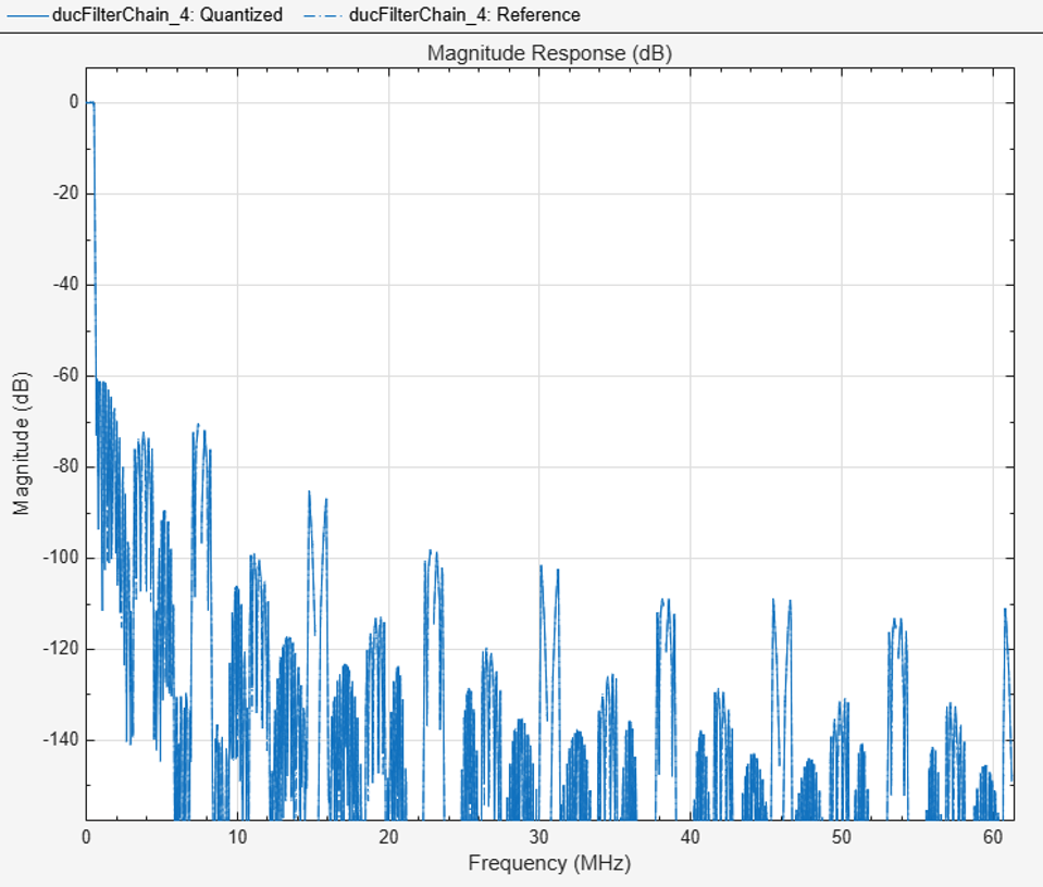
Redefine the ducFilterChain cascade object to include the fixed-point properties of the individual filters. Then use filterAnalyzer to analyze the entire filter chain and confirm that the quantized DUC still meets the specification.
ducFilterChain = dsp.FilterCascade(lowpassFilt,hbFilt,compFilt,cicFilt,GainCorr);
ducPlots.quantizedDUCResponse = filterAnalyzer(ducFilterChain, ...
    SampleRates=FsIn*64, ...
    Arithmetic='fixed');
HDL-Optimized Simulink Model
The next step in the design flow is to implement the DUC in Simulink using blocks that support HDL code generation.
Model Configuration
The model relies on variables in the MATLAB workspace to configure the blocks and settings. The filter blocks are configured by using the filter chain objects defined earlier in the example.
The input to the DUC comes from the ducIn variable. For now, assign a dummy value for ducIn so that the model can compute its data types. During testing, ducIn provides input data to the model.
ducIn = 0;
The outputFrame parameter sets the frame size of the output based on the DAC requirement. outputFrame affects the input vector size and valid sample spacing, and it should be a power of two. Using vector input and implementing parallel FPGA operations to achieve higher throughput is referred to as super-sample processing.
outputFrame = 4;
Model Structure
This figure shows the top level of the DUC Simulink model. The model imports the ducIn variable from the MATLAB workspace by using a Signal From Workspace block, converts the signal to 16-bit values, and applies the signal to the DUC. The design is single rate, and uses a valid signal to convey the rate change from block to block. To simulate the input running 64 times slower than the clock, it is upsampled by 64 with zero insertion. You can generate HDL code from the HDL_DUC subsystem.
modelName = 'DUCforLTEHDL';
open_system(modelName);
set_param(modelName,'Open','on');
The DUC implementation is inside the HDL_DUC subsystem.
set_param([modelName '/HDL_DUC'],'Open','on');
Filter Block Parameters
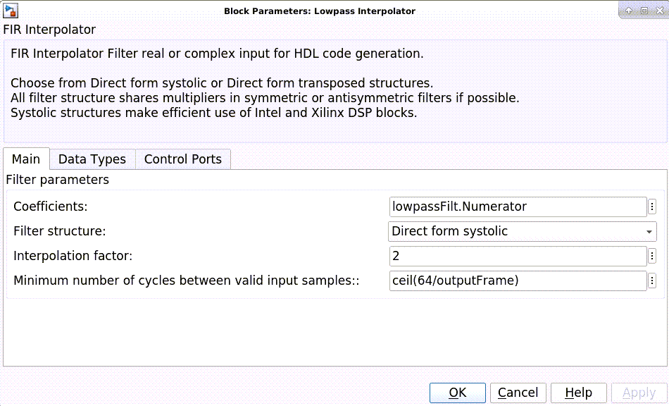
All of the filters are configured to inherit the coefficients of the corresponding System objects. Each block also has a "Minimum number of cycles between valid input" parameter that is used to optimize the resulting HDL code. The lowpass, halfband, and CIC compensation filters have cycles between valid inputs that can be used for resource sharing - 64, 32, and 16 cycles, respectively.
The FIR Interpolator block is fully serial when "Minimum number of cycles between valid input" is greater than or equal to length(Numerator)/(InterpolationFactor*length(Numerator). In some cases this can cause valid data to be produced faster than the next block can accept it. For example, when the output frame size is 2, then the "Minimum number of cycles between valid input" is set to 16 on the halfband filter, however the filter only has 11 taps, and therefore sharing is set to length(Numerator)/(InterpolationFactor*length(Numerator) = 12. Seeing as we are interpolating by 2, new output data will appear every 6 cycles. The next block in the chain (CIC compensation interpolator) expects valid data every 8 cycles which is greater than the 6 cycles at the input, therefore it is forced to drop data. To ensure that we have enough cycles between valid output samples, insert padding zeroes for each set of FIR Interpolator coefficients when required:
lowpassFilt.Numerator = [lowpassFilt.Numerator,zeros(1,ceil(64/(outputFrame)) -length(lowpassFilt.Numerator))];
hbFilt.Numerator = [hbFilt.Numerator,zeros(1,ceil(64/(2*outputFrame)) -length(hbFilt.Numerator))];
compFilt.Numerator = [compFilt.Numerator,zeros(1,ceil(64/(4*outputFrame)) -length(compFilt.Numerator))];
For example, because the sample rate of the input to the Lowpass Interpolation block is Fclk/64, 64 clock cycles are available to process each input sample.
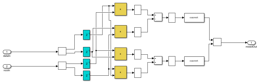
The first filter interpolates by 2. Each polyphase branch is implemented by a separate FIR Filter. Because the number of cycles between valid input samples is greater than 1, each FIR is implemented using the partly serial systolic architecture. The filter has 69 coefficients in total, and after polyphase decomposition each branch has 35 coefficients. There are 64 cycles available for sharing, so each branch is implemented with a fully serial FIR. With complex input, each branch uses 2 multipliers, for a total of 4 multipliers in this filter.
The second filter is a halfband interpolator. This filter can also take advantage of cycles between valid input to perform resource sharing. These cycles are available because each interpolator output has idle cycles between valid samples. The first filter has 64 cycles and interpolates by 2. Therefore, it will output data every 32 cycles. The second filter has 6 coefficients per polyphase branch and so it can be implemented as a fully serial FIR. In this filter, the second branch only contains one non-zero coefficient, and it is a power of 2. The FIR Interpolator block implements this branch as a shift rather than a multiplier. The second filter then has only 2 multipliers.
The third filter is a CIC compensation filter which interpolates by 2. It has 32 coefficients in total, which we specified when designing the filter. The filter is implemented using 2 fully serial complex FIRs, giving a total of 4 multipliers for this filter.
Gain Correction
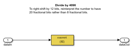
The gain correction divides the output by 4096, which is equivalent to shifting right by 12 bits. Because the input and output signals of the gain correction each are expressed with 18 bits, the model implements this shift by reinterpreting the data type of the output signal. The Conversion block reinterprets the 12-bit number to have 20 fractional bits rather than 8 fractional bits.
set_param([modelName '/HDL_DUC/Gain Correction'],'Open','on');
NCO Block Parameters
The NCO block generates a complex phasor at the carrier frequency. This signal goes to a mixer that multiplies the phasor with the output signal. The output of the mixer is sampled at 122.88 Msps.
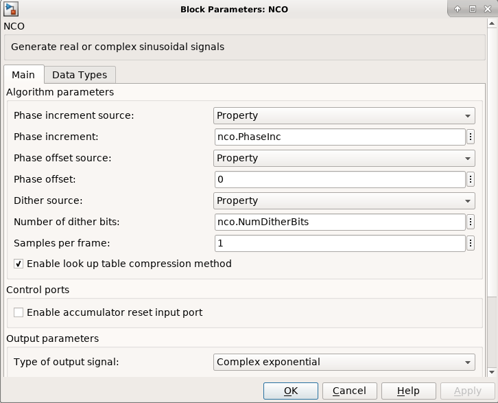
Specify the desired frequency resolution, then calculate the number of accumulator bits required to achieve the desired resolution, and define the number of quantized accumulator bits. The NCO uses the quantized output of the accumulator to address the sine lookup table. Also compute the phase increment the NCO must use to generate the specified carrier frequency. The NCO applies phase dither to the accumulator bits that are removed during quantization.
nco.Fd = 1;
nco.AccWL = nextpow2(FsIn*64/nco.Fd) + 1;
nco.QuantAccWL = 12;
nco.PhaseInc = round((Fc*2^nco.AccWL)/(FsIn*64));
nco.NumDitherBits = nco.AccWL-nco.QuantAccWL;
The NCO block in the model is configured with the parameters defined in the nco structure. This figure shows the NCO block parameters dialog.
Mixer
The Mixer subsystem performs a complex multiply of the filter output and NCO.
set_param([modelName '/HDL_DUC/Mixer'],'Open','on');
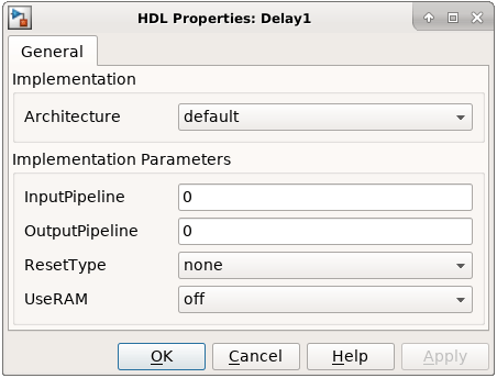
To map the mixer to DSP slices on FPGA, the mixer is pipelined and the blocks have specific settings. The delay blocks in the mixer are configured to have reset turned off as shown in the image. There are 2 pipeline stages at the input, 1 between the multiplier and adder, and another post-adder. Also, the multipliers and adders are configured to use full-precision output. These blocks use Floor rounding method, and the saturate on overflow logic is disabled.
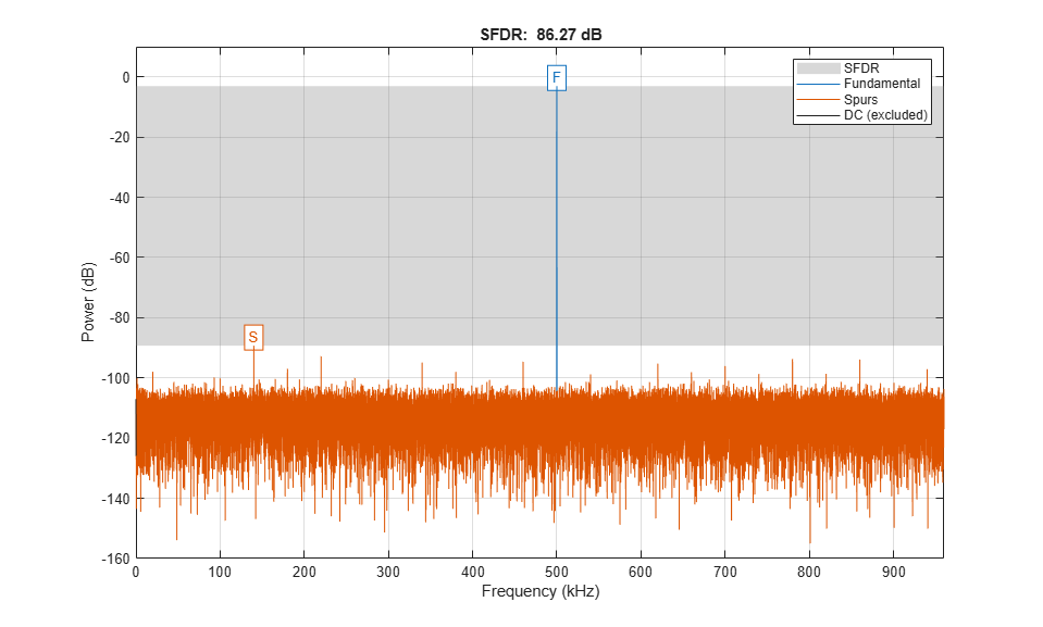
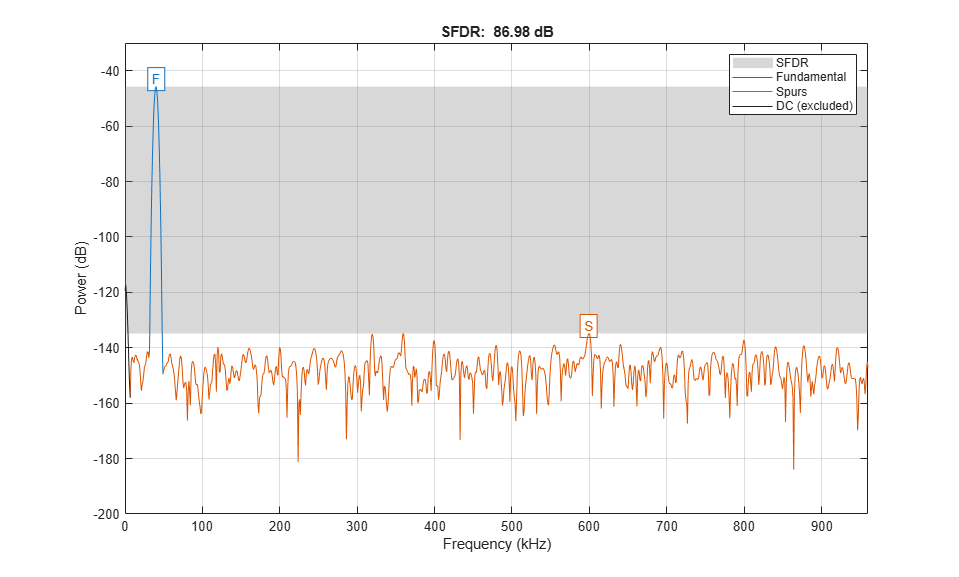
Sinusoid on Carrier Test
To test the DUC, pass a 40kHz sinusoid through the DUC and modulate the output signal onto the carrier frequency. Demodulate and resample the signal. Then measure the spurious free dynamic range (SFDR) of the resulting tone and the SFDR of the NCO output.
% Initialize random seed before executing any simulations.
rng(0);

% Generate a 40kHz test tone.
ducIn = DUCTestUtils.GenerateTestTone(40e3);

% Upconvert the test signal with the floating-point DUC.
ducTx = DUCTestUtils.UpConvert(ducIn,FsIn*64,Fc,ducFilterChain);
release(ducFilterChain);

% Down convert the output of DUC.
ducRx = DUCTestUtils.DownConvert(ducTx,FsIn*64,Fc);

% Upconvert the test signal by running the fixed-point Simulink model.
simOut = sim(modelName);

% Downconvert the output of DUC.
simTx = simOut.ducOut;
simRx = DUCTestUtils.DownConvert(simTx,FsIn*64,Fc);

% Measure the SFDR of the NCO, floating point DUC, and fixed-point DUC outputs.
results.sfdrNCO = sfdr(real(simOut.ncoOut),FsIn);
results.sfdrFloatDUC = sfdr(real(ducRx),FsIn);
results.sfdrFixedDUC = sfdr(real(simRx),FsIn);

disp('SFDR Measurements');
disp(['   Floating-point DUC SFDR: ',num2str(results.sfdrFloatDUC) ' dB']);
disp(['   Fixed-point NCO SFDR: ',num2str(results.sfdrNCO) ' dB']);
disp(['   Fixed-point DUC SFDR: ',num2str(results.sfdrFixedDUC) ' dB']);
fprintf(newline);

% Plot the SFDR of the NCO and fixed-point DUC outputs.
ducPlots.ncoOutSDFR = figure;
sfdr(real(simOut.ncoOut),FsIn);

ducPlots.ducOutSDFR = figure;
sfdr(real(simRx),FsIn);
SFDR Measurements
   Floating-point DUC SFDR: 287.9207 dB
   Fixed-point NCO SFDR: 86.2747 dB
   Fixed-point DUC SFDR: 86.9766 dB
LTE Signal Test
You can use an LTE test signal to perform more rigorous testing of the DUC. Generate a standard-compliant LTE waveform by using LTE Toolbox™ functions. Then, upconvert the waveform with the DUC model. Use LTE Toolbox functions to measure the error vector magnitude (EVM) of the resulting signals.
rng(0);
% Execute this test only if you have the LTE Toolbox product.
if license('test','LTE_Toolbox')

    % Generate an LTE test signal by using LTE Toolbox functions.
    [ducIn, sigInfo] = DUCTestUtils.GenerateLTETestSignal();

    % Upconvert the signal with the floating-point DUC and modulate onto carrier.
    ducTx = DUCTestUtils.UpConvert(ducIn,FsIn*64,Fc,ducFilterChain);
    release(ducFilterChain);

    % Add noise to the transmit signal.
    ducTxAddNoise = DUCTestUtils.AddNoise(ducTx);

    % Downconvert the received signal.
    ducRx = DUCTestUtils.DownConvert(ducTxAddNoise,FsIn*64,Fc);

    % Upconvert the signal by using the Simulink model.
    simOut = sim(modelName);

    % Add noise to the transmit signal.
    simTx = simOut.ducOut;
    simTxAddNoise = DUCTestUtils.AddNoise(simTx);

    % Downconvert the received signal.
    simRx = DUCTestUtils.DownConvert(simTxAddNoise,FsIn*64,Fc);

    results.evmFloat = DUCTestUtils.MeasureEVM(sigInfo,ducRx);
    results.evmFixed = DUCTestUtils.MeasureEVM(sigInfo,simRx);

    disp('LTE EVM Measurements');
    disp(['   Floating-point DUC RMS EVM: '  num2str(results.evmFloat.RMS*100,3) '%']);
    disp(['   Floating-point DUC Peak EVM: ' num2str(results.evmFloat.Peak*100,3) '%']);
    disp(['   Fixed-point DUC RMS EVM: '     num2str(results.evmFixed.RMS*100,3) '%']);
    disp(['   Fixed-point DUC Peak EVM: '    num2str(results.evmFixed.Peak*100,3) '%']);
    fprintf(newline);

end
LTE EVM Measurements
   Floating-point DUC RMS EVM: 0.813%
   Floating-point DUC Peak EVM: 2.53%
   Fixed-point DUC RMS EVM: 0.816%
   Fixed-point DUC Peak EVM: 2.81%
HDL Code Generation and FPGA Implementation
To generate the HDL code for this example you must have the HDL Coder™ product. Use the makehdl and makehdltb commands to generate HDL code and an HDL test bench for the HDL_DUC subsystem. The DUC was synthesized on an AMD® Zynq®-7000 ZC706 evaluation board. The table shows the post place-and-route resource utilization results for outputFrame of size 4. The design met timing with a clock frequency of 335 MHz.
T = table(...
    categorical({'LUT'; 'LUTRAM'; 'FF'; 'BRAM'; 'DSP'}),...
    categorical({'4708'; '654'; '6849'; '2'; '32'}),...
    'VariableNames',{'Resource','Usage'})
T =

  5×2 table

    Resource    Usage
    ________    _____

     LUT        4708
     LUTRAM     654
     FF         6849
     BRAM       2
     DSP        32
See Also
FIR Interpolator | CIC Interpolator | NCO