音叉の線形解析

この例では、音叉の構造モデルを線形化して、その腕の 1 本にインパルスが加えられたときの時間応答と周波数応答を計算する方法を説明します。この負荷により、腕の横振動と持ち手の縦振動が同じ周波数で発生します。構造モデルの詳細については、Structural Dynamics of Tuning Fork (Partial Differential Equation Toolbox)を参照してください。

この例には、Partial Differential Equation Toolbox™ ソフトウェアが必要です。

音叉の構造モデル

Partial Differential Equation Toolbox を使用して、音叉の構造モデルを作成します。

createpde (Partial Differential Equation Toolbox)を使用して構造モデルを作成します。

model = createpde(structural="transient-solid");

音叉の形状をインポートしてプロットします。

importGeometry(model,"TuningFork.stl");
figure
pdegplot(model)

ヤング率、ポアソン比、質量密度を指定して、線形弾性材料の動作をモデル化します。すべての物理特性を一貫した単位で指定します。

E = 210E9;
nu = 0.3;
rho = 8000;
structuralProperties(model,YoungsModulus=E, ...
                           PoissonsRatio=nu, ...
                           MassDensity=rho);
generateMesh(model,Hmax=0.005);

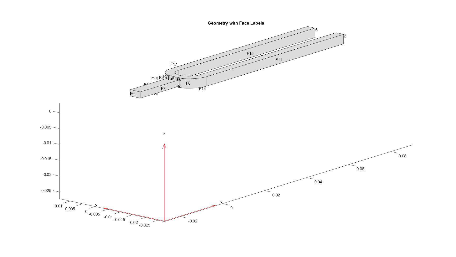
面のラベルを付けて形状をプロットし、境界の制約と負荷を適用する面を特定します。

figure(units="normalized",outerposition=[0 0 1 1])
pdegplot(model,FaceLabels="on")
view(-50,15)
title("Geometry with Face Labels")

腕の振動の最初のモードは約 2926 rad/s です。この値は、モード解析 (Structural Dynamics of Tuning Fork (Partial Differential Equation Toolbox)を参照)、またはこの例の線形解析の節で示すボード線図から判断できます。

対応する振動の周期を計算します。

T = 2*pi/2926;

境界条件を追加して、腕にインパルスを加えたときの剛体の動きを抑制します。通常、音叉は手で持つかテーブルに置いて使います。この境界条件の簡易的な近似として、腕と持ち手 (面 21 と 22) の交差部分近くの領域を固定します。

structuralBC(model,Face=[21,22],Constraint="fixed");

腕に対するインパルス負荷をモデル化するには、structuralBoundaryLoad (Partial Differential Equation Toolbox)を使用して、振動の基本周期 T の 2% にわたって圧力負荷を加えます。この非常に短い圧力パルスを使用することで、確実に音叉の基本モードだけが励起されるようになります。ラベル Pressure を指定し、この負荷を線形化の入力として使用します。

Te = 0.02*T;
structuralBoundaryLoad(model,Face=11,Pressure=5e6,EndTime=Te,Label="Pressure");

structuralIC (Partial Differential Equation Toolbox)を使用してモデルの初期条件を設定します。

structuralIC(model,Displacement=[0;0;0],Velocity=[0;0;0]);

構造モデルの線形化

この音叉モデルで、腕に対する圧力負荷から腕の先端 (面 12) の y 変位と持ち手 (面 6) の x 変位への線形モデルを取得します。

そのためには、最初に構造モデルについて線形化されるモデルの入出力を指定します。ここでは、入力はstructuralBoundaryLoad (Partial Differential Equation Toolbox)で指定された圧力であり、出力は面 12 の y 自由度と面 6 の x 自由度です。

linearizeInput(model,"Pressure");
linearizeOutput(model,Face=12,Component="y");
linearizeOutput(model,Face=6,Component="x");

次に、linearize (Partial Differential Equation Toolbox) コマンドを使用して mechss モデルを抽出します。

sys = linearize(model)

Sparse continuous-time second-order model with 28 outputs, 1 inputs, and 4926 degrees of freedom.
Model Properties

Use "spy" and "showStateInfo" to inspect model structure. 
Type "help mechssOptions" for available solver options for this model.

線形化されたモデルで、sys.OutputGroup を使用して、各面に関連付けられている出力を特定します。

sys.OutputGroup

ans = struct with fields:
    Face12_y: [1 2 3 4 5 6 7 8 9 10 11 12 13]
     Face6_x: [14 15 16 17 18 19 20 21 22 23 24 25 26 27 28]

各出力グループから 1 つのノードを選択して、1 つの入力と 2 つの出力をもつモデルを作成します。

sys = sys([1,14],:)

Sparse continuous-time second-order model with 2 outputs, 1 inputs, and 4926 degrees of freedom.
Model Properties

Use "spy" and "showStateInfo" to inspect model structure. 
Type "help mechssOptions" for available solver options for this model.

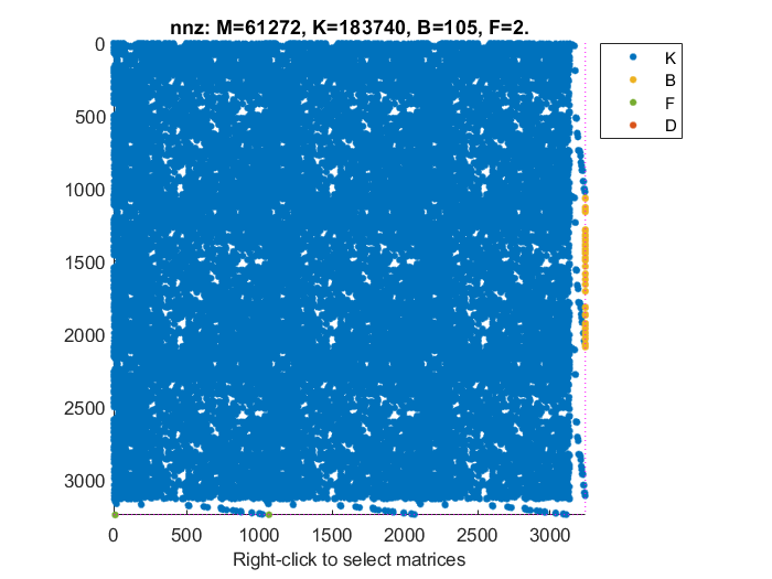
sys.OutputName = {'y tip','x base'};

結果のモデルは次の方程式のセットで定義されます。

$$\mathit{M}\ddot{\mathit{q}}+\mathit{K}\mathit{q}=\mathit{B}\times \mathrm{Pressure}$$

$$\mathit{y}=\mathit{F}\mathit{q}$$

spyを使用して mechss モデル sys のスパース性を可視化します。

figure
spy(sys)

線形解析

並列計算を有効にして、'tfbdf3' を微分代数方程式 (DAE) ソルバーとして選択します。

sys.SolverOptions.UseParallel = true;
sys.SolverOptions.DAESolver = "trbdf3";

bode を使用して、このモデルの周波数応答を計算します。

w = logspace(3,6,1000); 
figure
bode(sys,w) 

Starting parallel pool (parpool) using the 'Processes' profile ...
04-Mar-2024 14:34:16: Job Queued. Waiting for parallel pool job with ID 1 to start ...
Connected to parallel pool with 6 workers.

grid
title("Frequency Response from Pressure to Y Tip and X Base")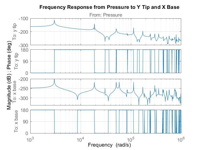

腕と持ち手が同じ周波数で振動していることがプロットで明確に示されています。最初のモードは約 2926 rad/s で、二次共振が約 6 倍の周波数で発生しています。

次に、lsim を使用して、基本モードの 20 周期について、線形化された音叉モデルのインパルス応答を取得します。サンプル間の圧力の線形内挿による誤差を制限するには、Te/10 のステップ サイズを使用します。圧力は時間間隔 [0 Te] で加えられます。

ncycle = 20;
Tf = ncycle*T;
h = Te/10;
t = 0:h:Tf;
u = zeros(size(t));    
u(t<=Te) = 5e6;
y = lsim(sys,u,t);

腕の先端の横方向変位と持ち手の縦方向変位をプロットします。

figure
plot(t,y(:,1))
title("Transverse Displacement at Tine Tip")
xlim([0,Tf])
xlabel("Time")
ylabel("Y-Displacement")
legend("Linearized model")

figure
plot(t,y(:,2))
title("Axial Displacement at End of Handle")
xlim([0,Tf])
ylabel("X-Displacement")
xlabel("Time")
legend("Linearized model")

参考

showStateInfo | spy | mechss | solve (Partial Differential Equation Toolbox) | structuralBC (Partial Differential Equation Toolbox) | structuralIC (Partial Differential Equation Toolbox) | createpde (Partial Differential Equation Toolbox) | linearize (Partial Differential Equation Toolbox) | linearizeInput (Partial Differential Equation Toolbox) | linearizeOutput (Partial Differential Equation Toolbox)

トピック

• スパース モデルの基礎