Improving an Engine Cooling Fan Using Design for Six Sigma Techniques
By Stuart Kozola, MathWorks and Dan Doherty, MathWorks
Engineers and scientists use a variety of approaches to improve or design quality into products. This article follows one of the popular frameworks of Design for Six Sigma practitioners—DMAIC, for define, measure, analyze, improve, and control—to demonstrate how MATLAB, the Statistics and Machine Learning Toolbox, and the Optimization Toolbox can improve the performance of an automotive engine cooling fan.
Defining the Problem with the Current Cooling Fan
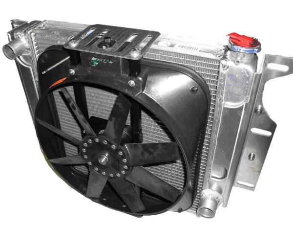
A key component of an engine’s cooling system is the cooling fan, which circulates air through the radiator to dissipate excess engine heat. Our cooling fan resembles the one shown in Figure 1. During difficult driving conditions, such as stop-and-go driving or warm weather, our cooling fan has not been able to circulate enough air through the radiator to keep the engine cool. We estimate that the cooling fan must pull in at least 875 ft3 per minute through the radiator to cool the engine adequately during difficult conditions. Our task is to determine if the current cooling fan design can be modified to deliver the required airflow without increasing the power consumption of the electric drive motor (120W) or modifying the surrounding interfaces. We will first measure the current cooling fan performance to establish a baseline, and then determine the design factors that we can alter to improve the fan’s performance.
Measuring the Performance of the Cooling Fan
To measure baseline performance, we collect data from the existing fan. Figure 2 shows a normal distribution fit to the data. The mean airflow for our existing fan is 842 ft3 per minute with a standard deviation of ± 2 ft3 per minute. Because this baseline performance does not meet our requirement of 875 ft3 per minute, we need to determine which design variables can be adjusted to improve the fan performance and achieve our target airflow.

Figure 2. Visual display of the data from the Distribution Fitting Tool in the Statistics and Machine Learning Toolbox. The data is best fit by a normal distribution curve.
Analyzing Factors that Affect Fan Performance
Factors that we can modify and analyze for effects on fan performance include the fan’s distance from the radiator, the tip clearance between the fan blades and the shroud, and the blade pitch angle. Other factors, such as the blade geometry and fan diameter, can not be changed due to time and space constraints. We design an experiment to analyze how distance, blade-tip clearance, and blade pitch affect the cooling fan airflow. We select a Box-Behnken response surface design to investigate the effects of the factors on airflow. Table 1 shows acceptable upper and lower bounds for the factors.
| Design Factors | Lower Bound | Upper Bound |
|---|---|---|
| Distance from radiator (inches) | 1 | 1.5 |
| Pitch angle (degrees) | 15 | 35 |
| Blade tip clearance (inches) | 1 | 2 |
Table 1. Selected range of design factors for testing.
The Box-Behnken design with three factors generates 15 testing combinations (13 unique plus 2 repeats), as shown in Table 2. We perform the 15 tests in random order, measuring airflow each time.
| Distance (Inches) | Pitch angle (degrees) | Blade-tip clearance (inches) | Mean airflow (ft3/minute) |
|---|---|---|---|
| 1.25 | 15 | 1.0 | 834 |
| 1.25 | 25 | 1.5 | 875 |
| 1.25 | 25 | 1.5 | 876 |
| 1.25 | 15 | 2.0 | 833 |
| 1.25 | 25 | 1.5 | 874 |
| 1.00 | 35 | 1.5 | 864 |
| 1.50 | 25 | 2.0 | 874 |
| 1.25 | 35 | 2.0 | 859 |
| 1.00 | 15 | 1.5 | 837 |
| 1.50 | 15 | 1.5 | 829 |
| 1.00 | 25 | 2.0 | 879 |
| 1.50 | 35 | 1.5 | 856 |
| 1.25 | 35 | 1.0 | 860 |
| 1.50 | 25 | 1.0 | 872 |
| 1.00 | 25 | 1.0 | 880 |
Table 2 shows that the airflow varies significantly for the different factor combinations.
We fit a quadratic model to estimate the linear, interaction, and quadratic effects of each factor. The quadratic model applied to our factors has the following form:
AF = B0 + B1X1 + B2X2 + B3X3 + B4X1X2 + B5X1X3 + B6X2X3 + B7X12 + B8X22 + B9X32,
where AF = airflow through radiator (ft3/min)
X1 = distance from radiator (inches)
X2 = fan pitch angle (degrees)
X3 = tip clearance between fan blades and shroud (inches).
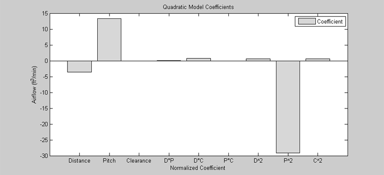
We use the regstats function from the Statistics and Machine Learning Toolbox to fit the quadratic model to the data and plot the coefficients to show which factors have the greatest effect on airflow (Figure 3).
s = regstats(TestResult, NormalizedFactors, 'quadratic');
bar(s.beta(2:10))
We normalize the factors over the range [-1, 1] to aid in identification of important factors and interactions. Without normalization, the coefficients of the factors will have to be adjusted for their unit values (e.g. ft3 per minute, inches, and degrees), making interpretation more difficult. Figure 3 shows how much each factor contributes to the total airflow. The large linear pitch coefficient indicates that a greater pitch angle generally results in higher airflow, while the large negative quadratic term indicates that the relationship between pitch angle and airflow is not strictly linear. Pitch is the dominant factor. The negative coefficient for distance reflects the fact that airflow increases when the fan is closer to the radiator. The small coefficients for the blade-tip clearance terms indicate that this factor has little effect on airflow.
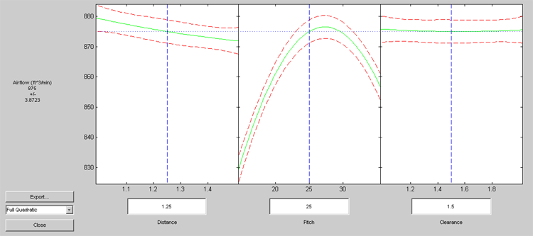
We can look at the relationship between multiple input variables and one output variable by generating a response surface plot. The Statistics and Machine Learning Toolbox includes the Response Surface Tool (rstool), which lets you interactively generate response surface plots from your data. Figure 4 shows a response surface plot of our airflow data generated from the quadratic model. The plots confirm what the coefficients already reveal: Effects of the blade pitch angle, distance, and blade-tip clearance are, respectively, nonlinear, linear, and negligible. Clearly, pitch has the strongest influence on airflow.

Improving the Cooling Fan Performance
We can use rstool to interactively adjust factor settings and estimate the optimal setting for the three factors that maximize the fan airflow. However, interactively estimating an optimal setting in this manner is time consuming and prone to error. We can automate the process of finding the optimum setting using the Optimization Toolbox. To find the optimum fan performance, we use the fmincon function from the Optimization Toolbox to solve our constrained optimization problem:
f = @(x) -x2fx(x, 'quadratic')*s.beta;
lb = [-1 -1 -1];
ub = [1 1 1];
x0 = [0 0 0];
[optfactors, fval] = fmincon(f,x0,[],[],[],[],lb,ub);
The optimization function, f, is the quadratic equation with the coefficients (s.beta) from the regression performed in regstats. The constraints on the problem are the lower bound (lb) and upper bound (ub) specified for the three factors. An initial condition, x0, is defined to start the optimization routine. Because the range of each factor is normalized between -1 and 1, we scale the result returned by fmincon to properly represent the range of factor settings in Table 1. The optimal airflow returned of 882 ft3 per minute occurs for the following factor values:
| Distance from radiator | 1 inch |
| Pitch angle | 27.3 degrees |
| Blade-tip clearance | 1 inch |
This result suggests the optimal configuration is a fan with 27.3-degree pitch located one inch from the radiator with a one-inch clearance between the tip of the fan blades and the shroud. Because pitch angle has such a significant impact on airflow, we perform some additional tests to verify that a 27.3-degree pitch angle is optimal.
We use a variable pitch test fan, varying the pitch angle in 0.5-degree increments from 15 to 35 degrees, and measure the airflow. We set the distance and blade-tip clearance at the optimal values. Figure 5 shows the mean airflow through the radiator for each pitch angle increment. A quadratic model fit to the test results estimates a maximum airflow of 882 ft3 per minute at a pitch angle of 27.5 degrees, which verifies the accuracy of the optimal pitch angle calculated in our optimization.

Figure 5. Test results from the variable pitch test fan. The quadratic model shows that the optimal pitch angle is around 27.5 degrees, corresponding to a maximum airflow of 882 ft3 per minute.
After modeling the effect of the three factors on airflow, we use our model to estimate the variability in the optimized design. Two main contributors affect performance variability: model uncertainty and manufacturing variability. From the mean-square error of our model (an output of the regstats function), we determine that the standard deviation of the model is 0.96 ft3 per minute. We use this value to estimate the effect of noise on our model. We expect the variability for the three design factors to be normally distributed with the following means and standard deviations:
| Real Values | Normalized Values | |
| Distance from radiator: | 1.00 +/- 0.05 inch | -1.00 +/- 0.25 |
| Blade pitch angle: | 27.3 +/- 0.5 degrees | 0.227 +/- 0.05 |
| Blade-tip clearance: | 1.00 +/- 0.05 inch | -1.00 +/- 0.125 |
| Model noise: | 0.00 +/- 0.96 ft3/min | Not applicable |
To estimate how variability affects our design, we use a Monte Carlo simulation. We define normally distributed data sets that represent model uncertainty and factor tolerances by using the normrnd function:
dist = normrnd(optfactors(1),0.25,[10000 1]);
pitch = normrnd(optfactors(2),0.05,[10000 1]);
clearance = normrnd(optfactors(3),0.125,[10000 1]);
noise = normrnd(0,0.96,[10000 1]);
The optfactors variable is a 3 × 1 vector containing the optimal factor settings from fmincon. We estimate the airflow for 10,000 test simulations that use random combinations of factor settings within the tolerance ranges described above. Figure 6 summarizes the result of our Monte Carlo simulation.

Figure 6. Normal distribution fitted to results of the Monte Carlo simulation.
The mean airflow is 882 ft3 per minute with a standard deviation of 2 ft3 per minute. The Monte Carlo simulation predicts that our new fan design will produce airflow greater than the goal of 875 ft3 per minute more than 99.999% of the time. Our model predicts that we should have no difficulty meeting our design objective if our assumptions about manufacturing variability are correct. We need to monitor and control the manufacturing and installation process to ensure that our design is achievable and maintainable in the presence of manufacturing and installation uncertainty.
Controlling Fan Manufacturing and Installation
We monitor and evaluate the manufacturing and installation process using statistical process control (SPC) techniques to ensure that our design works in practice. Figure 7 shows the first 30 days of production data for our new cooling fan, produced at a rate of five cooling fans per day. According to the results, our manufacturing process is in statistical control, as indicated by the absence of violations of control limits or nonrandom patterns in the data over time.

Figure 7. Statistical Process Control (SPC) charts (X-bar and S) for a 30-day period. Upper and lower control limits (UCL and LCL) are ± three standard deviations from the mean.
Summary
We used MATLAB, the Statistics and Machine Learning Toolbox, and the Optimization Toolbox to improve the performance of an engine cooling fan through a Design for Six Sigma DMAIC approach. Our initial fan did not circulate enough air through the radiator to keep the engine cool during difficult conditions. We designed an experiment to investigate the effect of three performance factors: fan distance from the radiator, blade-tip clearance, and blade pitch angle. We used our test data to estimate optimum values for each factor, resulting in a design that produced airflows beyond our goal of 875 ft3 per minute. Simulations verify that the new design should produce airflow according to our specifications in more than 99.999% of the fans manufactured.
Published 2006

