メインコンテンツ
結果:
Earlier this year a bunch of MATLAB users got together to talk about their hobbies in a lightning talk format.
- Using "UIHTML" to create app components and Lightning
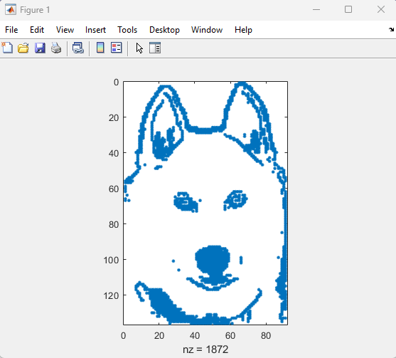
- Creating generative art with MATLAB
- Making MATLAB run on the Steam Deck (it was a wager)
Do you use MATLAB for hobbies?
Are there Matlab features which intend to satisfy your needs but fail in certain critical areas, forcing you to abandon them completely in favor of your own version or a 3rd party alternative? Perhaps these features are starting to improve with new Matlab releases, but not quickly enough? Share your own frustrations in the comments below.
Here are two of mine:
1. volumeViewier
volumeViewer is 6 years old now. It is fine when you only need to view one 3D image at a time, but I never do. In my work, I am putting several images side-by-side for visual comparison. For such work, you need to be able to programmatically change axis limits and grayscale and use linkprop to reflect these changes across all the images. With 2D image comparison, all that is possible, but volumeViewer supports none of those things. So, I resort to my own 3D viewer
2.Tomographic projection commands RADON and FANBEAM
These commands are provided in the Image Processing Toolbox seemingly for no other reason than to support homework exercises for people taking introductory tomographic imaging courses. They fail in a number of ways for people who need to do serious tomographic imaging work, producing artifacts or nonlinear effects which shouldn't be there. See for example Why isn't FANBEAM linear? or Radon Transform works unexpectedly. Moreover, the toolbox still provides tomographic projectors only for 2D imaging not 3D, even though 64-bit RAM has made volumetric imaging commonplace in Matlab for at least 10 years. Luckily, there are now freely available 3rd party alternatives like TIGRE.
Halloween Analysis of Many Aspects of Halloween Headquarters and Effects on USA
(Note to Chistopher: I used a simple ESP8266 generating random numbers for fields 1 thru 7, (0 to 100, 4000, 127, 30, 45, 200,000, 50,000) and 0 to 1 for field 8. And a couple of real sensor inputs.
Have you ever learned that something you were doing manually in MATLAB was already possible using a built-in feature? Have you ever written a function only to later realize (or be told) that a built-in function already did what you needed?
Two such moments come to mind for me.
1. Did you realize that you can set conditional breakpoints? Neither did I, until someone showed me that feature. To do that, open or create a file in the editor, right click on a line number for any line that contains code, and select Set Conditional Breakpoint... This will bring up a dialog wherein you can type any logical condition for which execution should be paused. Before I learned about this, I would manually insert if-statements during debugging. Then, after fixing each bug, I would have to delete those statements. This built-in feature is so much better.
2. Have you ever needed to plot horizontal or vertical lines in a plot? For the longest time, I would manually code such lines. Then, I learned about xline() and yline(). Not only is less code required, these lines automatically span the entire axes while zooming, panning, or adjusting axis limits!
Share your own Aha! moments below. This will help everyone learn about MATLAB functionality that may not be obvious or front and center.
(Note: While File Exchange contains many great contributions, the intent of this thread is to focus on built-in MATLAB functionality.)
The carot symbol on my keyboard (ˆ shift+6) doesn't work on matlab. Matlab doesn't recognize it so I can't write any equation with power symbol. I tried every possible solution on the web and it doesn't work. even in the character viewer I don't have any result when I search ''caret".
Exciting news for students! 🚀Simulink Student Challenge 2023 is live! Unleash your engineering skills and compete for exciting rewards. Submission deadline is December 12th, 2023!

In the past year, we've witnessed an exponential growth of ChatGPT and other Generative AI tools. AI has quickly become a transformative force across industries, from tech giants to small startups, and even community sites like ours. For instance, Stack Overflow announced its plan to leverage AI tools to draft a question or tag content; Quora built a ChatGPT bot to answer questions; and GitHub is piloting the AI tool for personalized content.

This trend in the community landscape makes me wonder what MATLAB Central community, especially in MATLAB Answers, can do to integrate AI and enhance the community.
Share with us your ideas in the comment session. Ideally one comment per idea, so that others can vote on a secific idea or have deeper discussions about it.
We launched the Discussions area with 6 channels, based on the existing types of content we see today in the MATLAB Central community.
I'm curious which channels you are most interested in participating, or which channels are missing.
Tell us your thoughts here!
Over the weekend I came across a pi approximation using durations of years and weeks (image below, Wolfram, eq. 89), accurate to 6 digits using the average Gregorian year (365.2425 days).

Here it is in MATLAB. I divided by 1 week at the end rather than multiplying by its reciprocal because you can’t divide a numeric by a duration in MATLAB (1/week).
weeks = @(n)n*days(7);
piApprox = ((years(13)-weeks(6))/years(13) + weeks(3)) / weeks(1)
% piApprox = 3.141593493469302
Here’s a breakdown
- The first argument becomes 12.885 yrs / 13 yrs or 0.99115
- Add three weeks: 0.99115 + 3 weeks = 21.991 days
- The reduced fraction becomes 21.991 days / 7 days
Now it looks a lot closer to the more familiar approximation for pi 22/7 but with greater precision!
Need help about FPGA Based VSC HVDC Real Time Simulation Model.
I'm in a community conference in Boston today and see what snacks we get! The organizer said it's a coincidence, but it's definitly a good idea to have them in our MathWorks community meetings.


(Sorry - it should be 2023b by now.)
spy

I'm curious how the community uses the hold command when creating charts and graphics in MATLAB. In short, hold on sets up the axes to add new objects to the axes while hold off sets up the axes to reset when new objects are added.
When you use hold on do you always follow up with hold off? What's your reasoning on this decision?
Can't wait to discuss this here! I'd love to hear from newbies and experts alike!
The way we've solved ODEs in MATLAB has been relatively unchanged at the user-level for decades. Indeed, I consider ode45 to be as iconic as backslash! There have been a few new solvers in recent years -- ode78 and ode89 for example -- and various things have gotten much faster but if you learned how to solve ODEs in MATLAB in 1997 then your knowledge is still applicable today.
In R2023b, there's a completely new framework for solving ODEs and I love it! You might argue that I'm contractually obliged to love it since I'm a MathWorker but I can assure you this is the real thing!
I wrote it up in a tutorial style on The MATLAB Blog https://blogs.mathworks.com/matlab/2023/10/03/the-new-solution-framework-for-ordinary-differential-equations-odes-in-matlab-r2023b/
The new interface makes a lot of things a much easier to do. Its also setting us up for a future where we'll be able to do some very cool algorithmic stuff behind the scenes.
Let me know what you think of the new functionality and what you think MathWorks should be doing next in the area of ODEs.
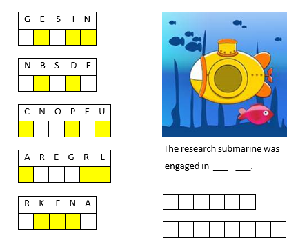
To solve the puzzle, first unscramble each of the words on the left. Then rearrange the letters in the yellow shaded boxes to complete the sentence on the right.

If you enjoyed this puzzle let me know with a like or in the comments below and I'll post more of them. Please don't post your answer, or any hints, and spoil it for those who come across this puzzle after you!! If you want to check your answer, you can messge me your guess through the link on my profile card (click on my name, Rena Berman, above and then on the envelope icon in the top right corner of the profile card that appears).
I am trying to make a simulink model to use a MPC to reduce power consumption of HVAC system in an electric vehicle during cool down from ambient temperature to a set point temperature. Any help regarding this would be appreciated
Hi Everyone,
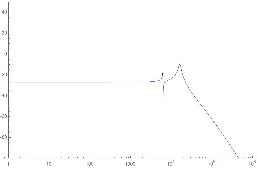
I have a high-order filter and I need to determinate its R,L,C values. In the simulation, the filter is unstable for some values. But I want to find values for stability of the filter. For second order system has some formulation between Q and phase margin so that it can be obtain the stability ciriteria to choose components.
My transfer function denominator is 5th order polynomial, and it is not possible to find roots in terms of R,L,C, Lm. I need to factor it like one 1th and two second order as shown in below.
D(s) = (1+s/wp) (1+s/wo1Q1 + (s/wo1)²) (1+s/wo2Q2 + (s/wo2)²)
Is there any methods to reduce order of transfer function?(Maybe, it can be possible for only in certain frequency range, can be renounced high-frequency )


Kindly help me correct this code to function properly. I am just learning MATLAB. i cannot get the output in abc frame. This is the code:
%----------- Define input and state parameters-----------------------------
clc
v_dc = 350; % DC input voltage in V
m = 0.841; % modulation index
C = 4000e-6; % DC buss capacitance in uf
L_1 = 2.5e-3; % Inverter side inductance in mH
L_2 = 2.5e-3; % Load side inductance in mH
L = 0; % load inductance
C_f = 10e-6; % filter capacitance in uf
R_f = 0.7; % damping resistance in ohms
R_L = 20; % load resistance in ohms
f_s = 10e3; % switching frequency
f = 60; % System frequency
R_s = 0.01; % Capacitance of the DC circuit
I_d = 8.594; % steady state current
w = 2*pi*f; % System angular Frequency
% Define initial steady state values
v_c = 349.4; i_d = 8.594; i_q = -0.213; v_df = 285; v_qf = -120; i_Ld = 8.594; i_Lq = 0.85;
%------------------S V P W M Generator-------------------------------------
% Define reference vector Uref
U_mag = m*v_dc/2; % Magnitude of Uref
% Define switching vectors
U1 = [v_dc/2;0]; % Vector Q1
U2 = [v_dc/4;sqrt(3)*v_dc/4]; % Vector Q2
U3 = [-v_dc/4;sqrt(3)*v_dc/4]; % Vector Q3
U4 = [-v_dc/2;0]; % Vector Q4
U5 = [-v_dc/4;-sqrt(3)*v_dc/4]; % Vector Q5
U6 = [v_dc/4;-sqrt(3)*v_dc/4]; % Vector Q6
% Define sector angles
theta1 = pi/6;
theta2 = pi/2;
theta3 = 5*pi/6;
theta4 = 7*pi/6;
theta5 = 3*pi/2;
theta6 = 11*pi/6;
% Define duty cycles for each switch using a for loop
for t=0:1/f_s:1/f % Time variable from 0 to one cycle of system frequency with steps of switching frequency
U_phase = w*t; % Phase of Uref (t is time variable)
U_alpha = U_mag*cos(U_phase); % Alpha component of Uref
U_beta = U_mag*sin(U_phase); % Beta component of Uref
if (0 <= U_phase) && (U_phase < theta1) % Sector 1
T1 = (sqrt(3)*U_beta + U_alpha)/(2*v_dc);
T2 = (-sqrt(3)*U_beta + U_alpha)/(2*v_dc);
T0 = 1 - T1 - T2;
d_a(round(t)+1) = T1 + T0/2;
d_b(round(t)+1) = T2 + T0/2;
d_c(round(t)+1) = T0/2;
elseif (theta1 <= U_phase) && (U_phase < theta2) % Sector 2
T3 = (sqrt(3)*U_beta - U_alpha)/(2*v_dc);
T2 = (sqrt(3)*U_beta + U_alpha)/(2*v_dc);
T0 = 1 - T3 - T2;
d_a(round(t)+1) = T0/2;
d_b(round(t)+1) = T2 + T0/2;
d_c(round(t)+1) = T3 + T0/2;
elseif (theta2 <= U_phase) && (U_phase < theta3) % Sector 3
T3 = (sqrt(3)*U_beta - U_alpha)/(2*v_dc);
T4 = (-sqrt(3)*U_beta - U_alpha)/(2*v_dc);
T0 = 1 - T3 - T4;
d_a(round(t)+1) = T0/2;
d_b(round(t)+1) = T0/2;
d_c(round(t)+1) = T3 + T0/2;
elseif (theta3 <= U_phase) && (U_phase < theta4) % Sector 4
T5 = (-sqrt(3)*U_beta + U_alpha)/(2*v_dc);
T4 = (-sqrt(3)*U_beta - U_alpha)/(2*v_dc);
T0 = 1 - T5 - T4;
d_a(round(t)+1) = T5 + T0/2;
d_b(round(t)+1) = T0/2;
d_c(round(t)+1) = T4 + T0/2;
elseif (theta4 <= U_phase) && (U_phase < theta5) % Sector 5
T5 = (-sqrt(3)*U_beta + U_alpha)/(2*v_dc);
T6 = (sqrt(3)*U_beta + U_alpha)/(2*v_dc);
T0 = 1 - T5 - T6;
d_a(round(t)+1) = T5 + T0/2;
d_b(round(t)+1) = T6 + T0/2;
d_c(round(t)+1) = T0/2;
elseif (theta5 <= U_phase) && (U_phase < theta6) % Sector 6
T1 = (sqrt(3)*U_beta + U_alpha)/(2*v_dc);
T6 = (sqrt(3)*U_beta - U_alpha)/(2*v_dc);
T0 = 1 - T1 - T6;
d_a(round(t)+1) = T1 + T0/2;
d_b(round(t)+1) = T0/2;
d_c(round(t)+1) = T6 + T0/2;
end
end
%-------------------------Define system matrices---------------------------
% Create Three-phase SVPWM VSI Inverter
% System matrix Nx-by-Nx matrix
A = [-1/(C*R_s),-sqrt(3)*m/(2*C),0,0,0,0,0;
sqrt(3)*m/(3*L_1),-R_f/(3*L_1),w,-1/(2*L_1),-sqrt(3)/(6*L_1),-R_f/(3*L_1),0;
0,-w,-R_f/(3*L_1),-sqrt(3)/(6*L_1),-1/(2*L_1),0,R_f/(3*L_1);
0,1/(2*C_f),-sqrt(3)/(6*C_f),0,w,-1/(2*C_f),sqrt(3)/(6*C_f);
0,sqrt(3)/(6*C_f),1/(2*C_f),-w,0,-sqrt(3)/(6*C_f),-1/(2*C_f);
0,R_f/(3*(L_2+L)),0,1/(2*(L_2+L)),sqrt(3)/(6*(L_2+L)),((-3*R_L-R_f)/(3*(L_2+L))),w;
0, 0, R_f/(3*(L_2+L)), -sqrt(3)/(6*(L_2+L)), 1/(2*(L_2+L)), -w, ((-3*R_L-R_f)/(3*(L_2+L)))];
% Define input matrix
B = [1/(C*R_s),-sqrt(3)*i_d/(2*C);d_a*v_dc,(sqrt(3)*v_c)/L_1;d_b*v_dc,0;d_c*v_dc,0;0,0;0,0;0,0]; % Nx-by-Nu input matrix
% Define output matrix
C = [0 1 0 0 0 0 0; % Ny-by-Nx matrix
0 0 1 0 0 0 0;
0 0 0 1 0 0 0;
0 0 0 0 1 0 0;
0 0 0 0 0 1 0;
0 0 0 0 0 0 1];
% Feedthrough matrix
D = zeros(6, 2); % Ny-by-Nu matrix
% create state-space model object
sys = ss(A,B,C,D);
% Define initial conditions and input
x0 = [v_c; i_d; i_q; v_df; v_qf; i_Ld; i_Lq]; % Initial state vector
t = 0:1e-6:0.5; % Time vector for simulation
u = repmat([v_dc;m],1,length(t)); % repeat u for each time step
% Simulate the system
[y, ~, x] = lsim(sys, u, t, x0);
% Extract the states
v_c_sim = x(:, 1);
i_d_sim = x(:, 2);
i_q_sim = x(:, 3);
v_df_sim = x(:, 4);
v_qf_sim = x(:, 5);
i_Ld_sim = x(:, 6);
i_Lq_sim = x(:, 7);
% Extract the outputs
v_abc_sim = y(:, 1:3);
i_abc_sim = y(:, 4:6);
v_dq_sim = y(:, 4:5);
i_dq_sim = y(:, 2:3);
% Plot the variables
figure;
subplot(4, 2, 1);
plot(t, v_c_sim);
xlabel('Time');
ylabel('v_c');
title('Capacitor Voltage');
subplot(4, 2, 2);
plot(t, i_d_sim);
xlabel('Time');
ylabel('i_d');
title('d-Axis Current');
subplot(4, 2, 3);
plot(t, i_q_sim);
xlabel('Time');
ylabel('i_q');
title('q-Axis Current');
subplot(4, 2, 4);
plot(t, v_df_sim);
xlabel('Time');
ylabel('v_df');
title('d-Component Filter Voltage');
subplot(4, 2, 5);
plot(t, v_qf_sim);
xlabel('Time');
ylabel('v_qf');
title('q-Component Filter Voltage');
subplot(4, 2, 6);
plot(t, i_Ld_sim);
xlabel('Time');
ylabel('i_Ld');
title('d-Axis Load Current');
subplot(4, 2, 7);
plot(t, i_Lq_sim);
xlabel('Time');
ylabel('i_Lq');
title('q-Axis Load Current');
% Perform coordinate transformation from dq frame to abc frame for currents
i_a_sim = cos(w*t)*i_d_sim - sin(w*t)*i_q_sim;
i_b_sim = cos(w*t - 2*pi/3)*i_d_sim - sin(w*t - 2*pi/3)*i_q_sim;
i_c_sim = cos(w*t + 2*pi/3)*i_d_sim - sin(w*t + 2*pi/3)*i_q_sim;
% Perform coordinate transformation from dq frame to abc frame for voltages
v_a_sim = cos(w*t)*v_df_sim - sin(w*t)*v_qf_sim;
v_b_sim = cos(w*t - 2*pi/3)*v_df_sim - sin(w*t - 2*pi/3)*v_qf_sim;
v_c_sim = cos(w*t + 2*pi/3)*v_df_sim - sin(w*t + 2*pi/3)*v_qf_sim;
Many thanks
The MATLAB Answers community is an invaluable resource for all MATLAB users, providing selfless assistance and support. However, with the emergence of AI-based chatbots, like chatGPT, there may be concerns about the future relevance and utility of the MATLAB Answer community. What are your thoughts?
