Stereo Disparity Using Semi-Global Block Matching
This example shows how to compute disparity between left and right stereo camera images using the Semi-Global Block Matching algorithm. This algorithm is suitable for implementation on an FPGA.
Distance estimation is an important measurement for applications in Automated Driving and Robotics. A cost-effective way of performing distance estimation is by using stereo camera vision. With a stereo camera, depth can be inferred from point correspondences using triangulation. Depth at any given point can be computed if the disparity at that point is known. Disparity measures the displacement of a point between two images. The higher the disparity, the closer the object.
This example computes disparity using the Semi-Global Block Matching (SGBM) method, similar to the disparity (Computer Vision Toolbox) function. The SGBM method is an intensity-based approach and generates a dense and smooth disparity map for good 3-D reconstruction. However, it is highly compute-intensive and requires hardware acceleration using FPGAs or GPUs to obtain real-time performance.
The example model presented here is FPGA-hardware compatible, and can therefore provide real-time performance.
Introduction
Disparity estimation algorithms fall into two broad categories: local methods and global methods. Local methods evaluate one pixel at a time, considering only neighboring pixels. Global methods consider information that is available in the whole image. Local methods are poor at detecting sudden depth variation and occlusions, and hence global methods are preferred. Semi-global matching uses information from neighboring pixels in multiple directions to calculate the disparity of a pixel. Analysis in multiple directions results in a lot of computation. Instead of using the whole image, the disparity of a pixel can be calculated by considering a smaller block of pixels for ease of computation. Thus, the Semi-Global Block Matching (SGBM) algorithm uses block-based cost matching that is smoothed by path-wise information from multiple directions.
Using the block-based approach, this algorithm estimates approximate disparity of a pixel in the left image from the same pixel in the right image. More information about stereo vision is available here. Two important parameters contribute to this algorithm: disparity levels and number of directions.
Disparity Levels: Disparity levels is a parameter used to define the search space for matching. As shown in the figure, the algorithm searches for each pixel in the left image from among D pixels in the right image. The values generated are D disparity levels for a pixel in the left image. The first D columns of the left image are unused because the corresponding pixels in the right image are not available for comparison. In the figure, w represents the width of the image and h is the height of the image. For a given image resolution, increasing the disparity level reduces the minimum distance to detect depth. Increasing the disparity level also increases the computation load of the algorithm. At a given disparity level, increasing the image resolution increases the minimum distance to detect depth. Increasing the image resolution also increases the accuracy of depth estimation. The number of disparity levels are proportional to the input image resolution for detection of objects at the same depth. This example supports disparity levels from 8 to 128 (both values inclusive). The example models and the explanation of the algorithm use 64 disparity levels. The models provided in this example can accept input images of any resolution.

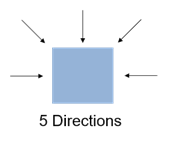
Number of Directions: In the SGBM algorithm, to optimize the cost function, the input image is considered from multiple directions. In general, accuracy of disparity result improves with increase in number of directions. This example analyzes five directions: left-to-right (A1), top-left-to-bottom-right (A2), top-to-bottom (A3), top-right-to-bottom-left (A4), and right-to-left (A5).
SGBM Algorithm
The SGBM algorithm takes a pair of rectified left and right images as input. The pixel data from the raw images may not have identical vertical coordinates because of slight variations in camera positions. Images need to be rectified before performing stereo matching. Rectifcation makes all epi-polar lines parallel to the horizontal axis and matches vertical coordinates of each corresponding pixel. For more details on rectification, see the rectifyStereoImages (Computer Vision Toolbox) function. The figure shows a block diagram of the SGBM algorithm, using five directions.

The SGBM algorithm implementation has three major modules: Matching Cost Calculation, Directional Cost Calculation, and Postprocessing.
Many methods are explored in the literature for computing matching cost. This example implementation uses the census transform as explained in [2]. This module can be divided into two steps: Center-Symmetric Census Transform (CSCT) of left and right images and Hamming Distance computation. First, the model computes the CSCT on each of the left and right images using a sliding window. For a given pixel, a 9-by-7 pixel window is considered around it. CSCT for the center pixel in that window is estimated by comparing the value of each pixel with its corresponding center-symmetric counterpart in the window. If the pixel value is larger than its corresponding center-symmetric pixel, the result is 1, otherwise the result is 0. The figure shows an example 9-by-7 window. The center pixel number is 31. The 0th pixel is compared to the 62nd pixel (blue), the 1st pixel is compared to the 61st pixel (red), and so on, to generate 31 results. Each result is a single bit output and the result of the whole window is arranged as a 31-bit number. This 31-bit number is the CSCT output for each pixel in both images.

In the Hamming Distance module, the CSCT outputs of the left and right images are pixel-wise XOR'd and set bits are counted to generate the matching cost for each disparity level. To generate D disparity levels, D pixel-wise Hamming distance computation blocks are used. The matching cost for D disparity levels at a given pixel position, p, in the left image is computed by computing the Hamming distance with (p to D+p) pixel positions in the right image. The matching cost, C(p,d), is computed at each pixel position, p, for each disparity level, d. The matching cost is not computed for pixel positions corresponding to the first D columns of the left image.
The second module of SGBM algorithm is directional cost estimation. In general, due to noise, the matching cost result is ambiguous and some wrong matches could have lower cost than correct ones. Therefore additional constraints are required to increase smoothness by penalizing changes of neighboring disparities. This constraint is realized by aggregating 1-D minimum cost paths from multiple directions. It is represented by aggregated cost from r directions at each pixel position, S(p,d), as given by

The 1-D minimum cost path for a given direction, L_r(p,d), is computed as shown in the equation.


As mentioned earlier, this example uses five directions for disparity computation. Propagation in each direction is independent. The resulting disparities at each level from each direction are aggregated for each pixel. Total cost is the sum of the cost calculated for each direction.
The third module of SGBM algorithm is Postprocessing. This module has three steps: minimum cost index calculation, interpolation, and a uniqueness function. Minimum cost index calculation finds the index corresponding to the minimum cost for a given pixel. Sub-pixel quadratic interpolation is applied on the index to resolve disparities at the sub-pixel level. The uniqueness function ensures reliability of the computed minimum disparity. A higher value of the uniqueness threshold marks more disparities unreliable. As a last step, the negative disparity values are invalidated and replaced with -1.
HDL Implementation
The figure shows the overview of the example model. The blocks leftImage and rightImage import a stereo image pair as input to the algorithm. In the Input subsystem, the Frame To Pixels block converts input images from the leftImage and rightImage blocks to a pixel stream and accompanying control signals in a pixelcontrol bus. The pixel stream is passed as input to the SGBMHDLAlgorithm subsystem which contains three computation modules described above: matching cost calculation, directional cost calculation, and postprocessing. The output of the SGBMHDLAlgorithm subsystem is a disparity value pixel stream. In the Output subsystem, the Pixels To Frame block converts the output to a matrix disparity map. The disparity map is displayed using the Video Viewer (Computer Vision Toolbox) block.
modelname = 'SGBMDisparityExample';
open_system(modelname);
set_param(modelname,'SampleTimeColors','off');
set_param(modelname,'Open','on');
set_param(modelname,'SimulationCommand','Update');
set(allchild(0),'Visible','off');

Matching Cost Calculation
The matching cost calculation is again separated into two parts: CSCT computation and Hamming distance calculation. CSCT is calculated on each 9-by-7 pixel window by aligning each group of pixels for comparison using Tapped Delay (Simulink) blocks, For Each Subsystem (Simulink) blocks and buffers. The input pixels are padded with zeros to allow CSCT computation for the corner pixels. The resulting stream of pixels is passed to the ctLogic subsystem. The figure shows the ctLogic subsystem which uses the Tapped Delay block to generate a group of pixels. The pixels are buffered for imgColSize cycles, where imgColSize is the number of pixels in an image line. A group of pixels that is aligned for comparison is generated from each row. The For Each block and Logical Operator (Simulink) block replicate the comparison logic for each pixel of the input vector size. To implement a 9-by-7 window, the model uses four such For Each blocks. The result generated by each For Each block is a vector which is further concatenated to form a vector of size 31-bits. After the Bit Concat (HDL Coder) block, the output data type is uint5. CSCT and zero-padding operations are performed separately on the left and right input images and the results are passed to the Hamming Distance subsystem.
open_system('SGBMDisparityExample/SGBMHDLAlgorithm/MatchingCost/CensusTransform/ctLogic','force');

In the Hamming Distance subsystem, the 65th result of the left CSCT is XOR'd with the 65th to 2nd results of the right CSCT. The set bits are counted to obtain Hamming distance. This distance must be calculated for each disparity level. The right CSCT result is passed to the enabledTappedDelay subsystem to generate a group of pixels which is then XOR'd with the left CSCT result using For Each block. The For Each block also counts the set bits in the result. The For Each block replicates the Hamming distance calculation for each disparity level. The result is a vector, with 64 disparity levels corresponding to each pixel. This vector is the Matching Cost, and it is passed to the Directional Cost subsystem.
open_system('SGBMDisparityExample/SGBMHDLAlgorithm/MatchingCost/HammDistA','force');

Directional Cost Calculation
The Directional Cost subsystem computes disparity at each pixel in multiple directions. The five directions used in the example are left-to-right (A1), top-left-to-bottom-right (A2), top-to-bottom (A3), top-right-to-bottom-left (A4), and right-to-left (A5). As the cost aggregation at each pixel in each direction is independent of each other, all five directions are implemented concurrently.
Each directional analysis is investigating the previous cost value with respect to the current cost value. The value of previous cost required to compute the current cost for each pixel depends on the direction under consideration. The figure shows the position of the previous cost with respect to the current cost under computation, for all five directions.

In the figure, the blue box indicates the position of the current pixel for which current cost values are computed. The red box indicates the position of the previous cost values to be used for current cost computation. For A1, the current cost becomes the previous cost value for the next computation when traversing from left to right. Thus, the current cost value should be immediately fed back to compute the next current cost, as described in [3]. For A2, when traversing from left to right, current cost value should be used as the previous cost value after imgColSize+1 cycles. Current cost values are hence buffered for cycles equal to imgColSize+1 and then fed back to compute the next current cost.
Similarly, for A3 and A4, the current cost values are buffered for cycles equal to imgColSize and imgColSize-1, respectively. However, for A5, when traversing from left to right, the previous cost value is not available. Thus, the direction of traversal to compute A5 is reversed. This adjustment is done by reversing the input pixels of each row. The current cost value then becomes the previous cost value for the next current cost computation, similar to A1.
The 1-D minimum cost path computes the current cost at d disparity position, using the Matching Cost value, the previous cost values at disparities d-1, d, and d+1, and the minimum of the previous cost values. The figure shows the minCostPath subsystem, which computes the current cost at a disparity position for a pixel.
open_system('SGBMDisparityExample/SGBMHDLAlgorithm/DirectionalCost/LeftToRight/lrSubsystem/minCostPath','force');

The For Each block replicates the minimum cost path calculation for each disparity level, for each direction. The figure shows the implementation of A1 for 64 disparity levels. As shown in the figure, 64 minimum cost path calculations are generated as represented by minCostPath subsystem. The matching cost is an input from the Hamming Distance subsystem. The current cost computed by the minCostPath subsystem is immediately fed back to itself as the previous cost values, for the next current cost computation. Thus, values for prevCost_d are now available. Values for prevCost_d-1 are obtained by shifting the 1st to 63rd fed-back values to the 2nd to 64th positions. The d-1 subsystem contains a Selector (Simulink) block that shifts the position of the values, and fills in zero at the 1st position.
Similarly, values for prevCost_d+1 position are obtained by shifting the 2nd to 64th feedback values to the 1st to 63rd position and inserting a zero at the 64th position. The current cost computed is also passed to the min block to compute the minimum value from the current cost values. This value is fed back to the minPrevCost input of the minCostPath subsystem. The next current cost is then computed by using the current cost values, acting as previous cost values, in the next cycle for A1. Since the minimum cost of disparity levels from the previous set is immediately needed for the current set, this feedback path is the critical path in the design.
open_system('SGBMDisparityExample/SGBMHDLAlgorithm/DirectionalCost/LeftToRight/lrSubsystem','force');

The current cost computations for A2, A3, and A4 are implemented in the same manner. Since the current cost value is not immediately required for these directions, there is a buffer in both feedback paths. This buffer prevents this feedback path from being the critical path in the design. The figure below shows the A3 implementation with a buffer in the feedback paths.
open_system('SGBMDisparityExample/SGBMHDLAlgorithm/DirectionalCost/TopToBottom/tbSubsystem','force');

The current cost calculation for A5 has additional logic to reverse the rows at input and again reverse the rows at output to match the pixel positions for the total cost calculation. A single buffer of imgColSize cycles achieves this reversal. Since all directions are calculated concurrently, the time required to reverse the rows must be compensated for on the other paths. Delay equivalent to 2*imgColSize cycles is introduced in the other four directions. To optimize resources, instead of buffering 64 values of matching cost for each pixel, the 31-bit result of CSCT is buffered. A separate Hamming Distance module is then required to compute matching cost for A5. This design reduces on-chip memory usage. The rows are reversed after the CSCT computation and matching cost is calculated using a separate Hamming Distance module that provides the Matching Cost input to A5. Also, dataAligner subsystem removes data discontinuity for each row before passing it to the Hamming Distance subsystem. This helps synchronize data at the time of aggregation. The current cost obtained from all five directions at each pixel are aggregated to obtain the total cost at each pixel. The total cost is passed to the Postprocessing subsystem.
Postprocessing
In the Postprocessing subsystem, the index of the minimum cost is calculated at each pixel position from 64 disparity levels by using MinMax (Simulink) blocks in a tree architecture. The index value obtained is the disparity of each pixel. Along with minimum cost index computation, the minimum cost value at the computed index, and the cost values at index-1 and index+1 are also computed. The Minimum_Cost_Index subsystem implements a tree architecture to compute a minimum value from 128 values. 64 disparity values are padded with 64 more values to make a vector of 128 values. The minimum value is found from this 128-value vector. If a vector with 128 values is available, no value is padded, and the vector is passed directly for minimum value calculation. A Variant Subsystem (Simulink) block selects between these options. Sub-pixel quadratic interpolation is then applied to the index to resolve disparity at the sub-pixel level. To ensure reliable disparity results, a uniqueness function is applied to the index calculated by the Min blocks. As a last step, invalid disparities are identified and replaced with -1.
Model Parameters
The model presented here takes Disparity levels and Uniqueness threshold as input parameters. Disparity levels must be an integer value from 8 to 128. The default value is 64. Higher disparity levels reduce the minimum distance detected. Also, for larger input image sizes, a larger disparity level helps better detect the depth of objects. The Uniqueness threshold must be a positive integer value, between 0 and 100. A typical range is from 5 to 15. A lower uniqueness threshold marks more disparities reliable. The default value of the Uniqueness threshold is 5.

Simulation and Results
The example model can be simulated by specifying a path for the input images in the leftImage and rightImage blocks. The example uses sample images of size 640-by-480 pixels. The figure shows a sample input image and the calculated disparity map. The model exports these calculated disparities and a corresponding valid signal to the MATLAB workspace, using variable names dispMap and dispMapValid respectively. The output disparity map is 576-by-480 pixels, since the first 64 columns are unused in the disparity computation. The unused pixels are padded with 0 in the Output subsystem to generate output image of size 640-by-480 as shown in Video Viewer. A disparity map with colorbar is generated using the commands shown below. Higher disparity values in the result indicate that the object is nearer to the camera and lower disparity values indicate farther objects.
dispMapValid = find(dispMapValid == 1);
disparityMap = (reshape(dispMap(dispMapValid(1:imgRowSize*imgColSize),:),imgColSize,imgRowSize))';
figure(); imagesc(disparityMap);
title('Disparity Map');
colormap jet; colorbar;


The example model is compatible to generate HDL code. You must have an HDL Coder™ license to generate HDL code. The design was synthesized for the Intel® Arria® 10 GX (115S2F45I1SG) FPGA. The table below shows resource utilization for three disparity level at different image resolutions. Considering one pair of stereo input images as a frame, the algorithm throughput is estimated by finding the number of clock cycles required for processing the current frame before the arrival of next frame. The core algorithm throughput, without overhead of buffering input and output data, is the maximum operating frequency divided by the minimum cycles required between input frames. For example, for 128 disparity levels and 1280-by-720 image resolution, the minimum cycles to process the input frame is 938,857 clock cycles/frame. The maximum operating frequency obtained for algorithm with 128 disparity levels is 61.69 MHz, the core algorithm throughput is computed as 65 frames per second.
% ==================================================================================
% |Disparity Levels        ||       64       ||       96       ||        128       |
% ==================================================================================
% |Input Image Resolution  ||    640 x 480   ||    960 x 540   ||     1280 x 720   |
% |ALM Utilization         ||   45,613 (11%) ||   64,225 (15%) ||    85,194 (20%)  |
% |Total Registers         ||     49,232     ||     64,361     ||      85,564      |
% |Total Block Memory Bits || 3,137,312 (6%) || 4,599,744 (9%) || 11,527,360 (21%) |
% |Total RAM Blocks        ||    264 (10%)   ||    409 (16%)   ||      741 (28%)   |
% |Total DSP Blocks        ||     65 (4%)    ||     97 (6%)    ||      129 (8%)    |
% ==================================================================================
References
[1] Hirschmuller H., Accurate and Efficient Stereo Processing by Semi-Global Matching and Mutual Information, International Conference on Computer Vision and Pattern Recognition, 2005.
[2] Spangenberg R., Langner T., and Rojas R., Weighted Semi-Global matching and Center-Symmetric Census Transform for Robust Driver Assistance, Computer Analysis of Images and Patterns, 2013.
[3] Gehrig S., Eberli F., and Meyer T., A Real-Time Low-Power Stereo Vision Engine Using Semi-Global Matching, International Conference on Computer Vision System, 2009.
See Also
Blocks
- Frame To Pixels | Variant Subsystem (Simulink) | Selector (Simulink) | Tapped Delay (Simulink) | For Each Subsystem (Simulink) | Bit Concat (HDL Coder) | Logical Operator (Simulink) | MinMax (Simulink)
Functions
disparity(Computer Vision Toolbox) |rectifyStereoImages(Computer Vision Toolbox)