Point Cloud Classification Using PointNet++ Deep Learning
This example shows how to classify 3-D objects in point cloud data by using a PointNet++ deep learning network.
Point cloud data is 3-D position information about objects in a scene, captured by sensors such as lidar sensors, radar sensors, and depth cameras. You can use point cloud data in autonomous driving and augmented reality applications, such as discriminating vehicles from pedestrians while planning the path of an autonomous vehicle. For example, you can use point cloud data to distinguish vehicles from pedestrians while planning the path of an autonomous vehicle. However, training robust classifiers with point cloud data is challenging due to sparse data, object occlusions, and sensor noise. Deep learning methods can address these challenges by learning robust feature representations directly from the data. PointNet++ [1] is a key deep learning method for classifying point cloud data.
This example trains a PointNet++ classifier on the Sydney Urban Objects data set [2]. This data set provides a collection of point cloud data acquired from an urban environment using a lidar sensor. The data set has 588 labeled objects from 14 different classes, such as car, pedestrian, and bus.
Download Data Set
Download and extract the Sydney Urban Objects data set to a temporary directory using the helperDownloadSydneyUrbanObjects helper function, attached to this example as a supporting file.
dataFolder = tempdir;
datapath = helperDownloadSydneyUrbanObjects(dataFolder);
Load Data
Load the training and test sets using the helperLoadSydneyUrbanObjectsData helper function. This function returns the fileDatastore objects trainDs and testDs from which to read point cloud files. This example uses the first three data folds for the training set and the fourth for the test set.
classNames = ["4wd","building","bus", ...
    "car","pedestrian","pillar","pole", ...
    "traffic lights","traffic sign", ...
    "tree", "truck","trunk","ute","van"];
trainFolds = 1:3;
testFolds = 4;
trainDs = helperLoadSydneyUrbanObjectsData(datapath,trainFolds,classNames);
testDs = helperLoadSydneyUrbanObjectsData(datapath,testFolds,classNames);
Read and display a sample point cloud from the training data set.
data = preview(trainDs);
ptCloud = data{1,1};
className = data{1,2};

figure
pcshow(ptCloud.Location,[0 1 0],MarkerSize=40,VerticalAxisDir="down")
xlabel("X")
ylabel("Y")
zlabel("Z")
title(className)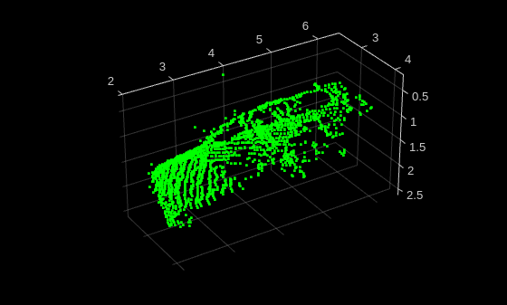
Perform Data Augmentation
Data augmentation improves network accuracy by adding more variety to the training data without actually increasing the number of labeled training samples. To perform data augmentation, you randomly transform a subset of your original training samples to generate new training samples. Use the transform function, referencing the helperAugmentPointCloud helper function defined at the end of this example, to perform operations such as:
Random scaling by 5%
Random rotation along the z-axis in the range [–45, 45] degrees
Random drop of 30% of the points
Random jitter of the point location with Gaussian noise
Random translation by [0.2, 0.2, 0.1] meters along the x-, y-, and z-axes, respectively
Note: To accurately measure the performance of a trained network, use test data that represents the original data, and do not include synthetic data. This example does not apply augmentation to the test data set.
rng(0)
trainDs = transform(trainDs,@helperAugmentPointCloud);
Display an augmented point cloud.
data = preview(trainDs);
ptCloud = data{1,1};
className = data{1,2};

figure
pcshow(ptCloud.Location,[0 1 0],MarkerSize=40,VerticalAxisDir="down")
xlabel("X")
ylabel("Y")
zlabel("Z")
title(className)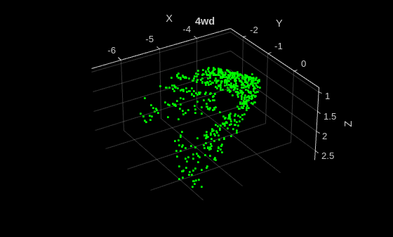
Create PointNet++ Classifier
Create a PointNet++ classification network by using the pointNetPlusClassifier function.
classifier = pointNetPlusClassifier("random",classNames);Specify Training Options
Use the Adam optimization algorithm to train the network. Use the trainingOptions function to specify the hyperparameters for training.
Note: To specify the PreprocessingEnvironment training option as "parallel", you must have a Parallel Computing Toolbox™ license.
numEpochs = 200;
miniBatchSize = 24;
options = trainingOptions("adam", ...
    InitialLearnRate=0.001, ...
    L2Regularization=1e-4, ...
    MaxEpochs=numEpochs, ...
    MiniBatchSize=miniBatchSize, ...
    LearnRateSchedule="piecewise", ...
    LearnRateDropFactor=0.7, ...
    LearnRateDropPeriod=20, ...
    Plots="training-progress", ...
    PreprocessingEnvironment="parallel", ...
    Shuffle="every-epoch", ...
    ResetInputNormalization=false, ...
    CheckpointFrequency=10, ...
    CheckpointFrequencyUnit="epoch", ...
    CheckpointPath=tempdir);
Train PointNet++ Classifier
To train the PointNet++ classifier, set the doTraining variable to true and use the trainPointNetPlusClassifier function. You can use a CPU or a GPU. Using a GPU requires Parallel Computing Toolbox™ and a CUDA® enabled NVIDIA® GPU. For more information, see GPU Computing Requirements (Parallel Computing Toolbox).
Instead of training the network, you can use a pretrained PointNet++ classifier by setting the doTraining variable to false.
doTraining = false;
if doTraining
    classifier = trainPointNetPlusClassifier(trainDs,classifier,options);
else
    classifier = pointNetPlusClassifier("sydney-urban");
end
Classify Point Cloud
Read a point cloud from the test sample, and run the trained classifier to get classes and scores.
testData = preview(testDs);
ptCloud = testData{1};
[classes,scores] = classify(classifier,ptCloud);
figure
pcshow(ptCloud.Location,[0 1 0],MarkerSize=40,VerticalAxisDir="down")
xlabel("X")
ylabel("Y")
zlabel("Z")
title(classes)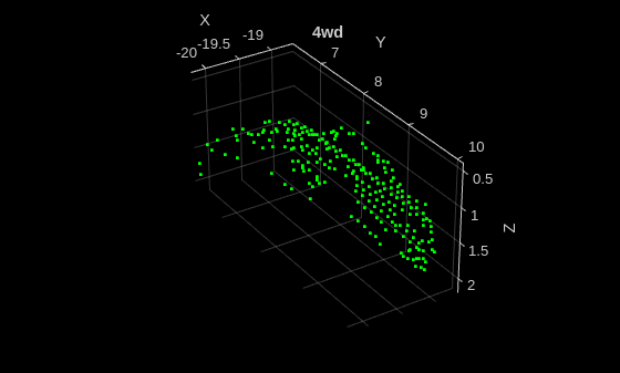
Evaluate Network
Run the classifier on the entire test data set.
[predClasses,scores] = classify(classifier,testDs);
Extract ground truth labels from the test datastore.
testLabelSet = transform(testDs,@(data)data{2});
trueClasses = readall(testLabelSet);
Compute a confusion matrix for the predicted and ground truth classes, and visualize it.
[cmat,order] = confusionmat(trueClasses,predClasses);
confusionchart(cmat,classNames);
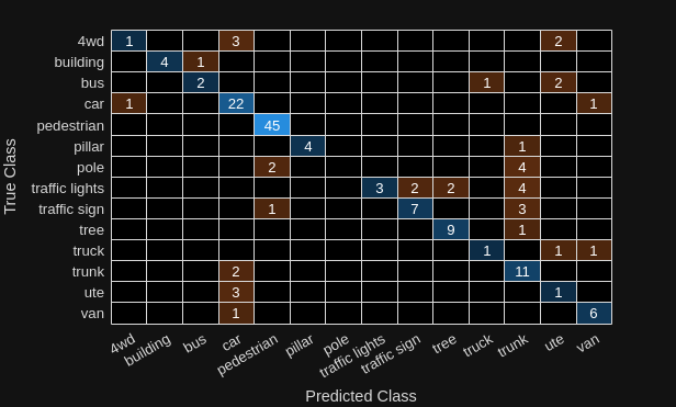
Calculate instance accuracy, which reflects the overall performance of the model across all classes.
instanceAccuracy = trace(cmat)*100/sum(cmat,"all");
fprintf("Instance Accuracy: %.2f%%n",instanceAccuracy)
Instance Accuracy: 74.84%
Calculate class accuracy, which reflects how well the model predicted each individual class.
classAccuracies = diag(cmat)./sum(cmat,2);
averageClassAccuracy = mean(classAccuracies)*100;
fprintf("Average Class Accuracy: %.2f%%n",averageClassAccuracy)
Average Class Accuracy: 58.42%
Supporting Functions
The helperAugmentPointCloudData function applies these augmentations to the data:
Random scaling by 5%
Random rotation along the z-axis in the range [–45, 45] degrees
Random drop of 30% of the points
Random jitter of the point location with Gaussian noise
Random translation by [0.2, 0.2, 0.1] meters along the x-, y-, and z-axes, respectively
function data = helperAugmentPointCloud(data)
ptCloud = data{1};
minAngle = -45;
maxAngle = 45;
theta = minAngle + rand(1,1)*(maxAngle - minAngle);
tform = randomAffine3d( ...
    Rotation=@()deal([0,0,1],theta), ...
    Scale=[0.95 1.05], ...
    XTranslation=[0 0.2], ...
    YTranslation=[0 0.2], ...
    ZTranslation=[0 0.2], ...
    XReflection=true, ...
    YReflection=true);
ptCloud = pctransform(ptCloud,tform);

% Randomly drop out 30% of the points.
if rand > 0.5
    ptCloud = pcdownsample(ptCloud,random=0.3);
end

if rand > 0.5
    % Jitter the point locations with Gaussian noise with a mean of 0 and
    % a standard deviation of 0.02 by creating a random displacement field.
    D = 0.02*randn(size(ptCloud.Location));
    ptCloud = pctransform(ptCloud,D);
end

data{1} = ptCloud;

end
The helperLoadSydneyUrbanObjectsData function creates a datastore for loading point cloud and label data from the Sydney Urban Objects data set.
function ds = helperLoadSydneyUrbanObjectsData(datapath,folds,classNames)

if nargin == 0
    return
end

if nargin < 2
    folds = 1:4;
end

datapath = string(datapath);
path = fullfile(datapath,"objects",filesep);

% Add folds to datastore.
foldNames{1} = importdata(fullfile(datapath,"folds","fold0.txt"));
foldNames{2} = importdata(fullfile(datapath,"folds","fold1.txt"));
foldNames{3} = importdata(fullfile(datapath,"folds","fold2.txt"));
foldNames{4} = importdata(fullfile(datapath,"folds","fold3.txt"));
names = foldNames(folds);
names = vertcat(names{:});

fullFilenames = append(path,names);
ds = fileDatastore(fullFilenames,ReadFcn=@(x)helperExtractTrainingData(x,classNames),FileExtensions=".bin");
end
The helperExtractTrainingData function extracts point cloud and label data from the Sydney Urban Objects data set.
function dataOut = helperExtractTrainingData(fname,classNames)

[pointData,intensity] = helperReadBinaryFiles(fname);

[~,name] = fileparts(fname);
name = string(name);
name = extractBefore(name,'.');
name = replace(name,'_',' ');

label = categorical(name,classNames);

dataOut = {pointCloud(pointData,Intensity=intensity) label};

end
References
[1] Qi, Charles R., Li Yi, Hao Su, and Leonidas J. Guibas. "PointNet++: Deep Hierarchical Feature Learning on Point Sets in a Metric Space." arXiv, 2017. https://doi.org/10.48550/ARXIV.1706.02413.
[2] de Deuge, Mark, Alastair Quadras, Calvin Hung, and Bertrand Douillard. "Unsupervised Feature Learning for Classification of Outdoor 3D Scans." In Australasian Conference on Robotics and Automation 2013 (ACRA 13). Sydney, Australia: ACRA, 2013.
See Also
pointNetPlusClassifier | trainPointNetPlusClassifier
Topics
- Get Started with PointNet++
- Lidar Object Detection Using Complex-YOLO v4 Network
- Lidar 3-D Object Detection Using PointPillars Deep Learning
- Data Augmentations for Lidar Object Detection Using Deep Learning
- Transfer Learning Using Voxel R-CNN for Lidar 3-D Object Detection
- Aerial Lidar Semantic Segmentation Using PointNet++ Deep Learning